Painting with Math: A Gentle Study of Raymarching

Snapshots of Math: demystifying the concept of Raymarching

If you're already familiar with Three.js or React Three Fiber 3D scenes, you most likely encountered the concepts of geometry, material, and mesh and maybe even built quite a few scenes with those constructs. Under the hood, rendering with them involves a technique called Rasterization, the process of converting 3D geometries to pixels on a screen.

Raymarching on the other hand, is an alternative rendering technique to render a 3D scene, without requiring geometries or meshes...

Marching rays

Raymarching consists of marching step-by-step alongside rays cast from an origin point (a camera, the observer's eye, ...) through each pixel of an output image until they intersect with objects in the scene within a set maximum number of steps. When an intersection occurs, we draw the resulting pixel.

That's the simplest explanation I could come up with. However, it never hurts to have a little visualization to go with the definition of a new concept! That's why I built the widget below illustrating:

• The step-by-step aspect of Raymarching: The visualizer below lets you iterate up to 13 steps.
• The rays cast from a single point of origin (bottom panel)
• and the intersections of those rays with an object resulting in pixels on the fragment shader (top panel)

Defining the World with Signed Distance Fields

The definition I just gave you above is only approximately correct. Usually, when working with Raymarching:

• We won't go step-by-step with a constant step distance along our rays. That would make the process very long.
• We also won't be relying on the intersection points between the rays and the object.

Instead, we will use Signed Distance Fields, functions that calculate the shortest distances between the points reached while marching alongside our rays and the surfaces of the objects in our scene. Relying on the distance to a surface lets us define the entire scene with simple math formulas ✨.

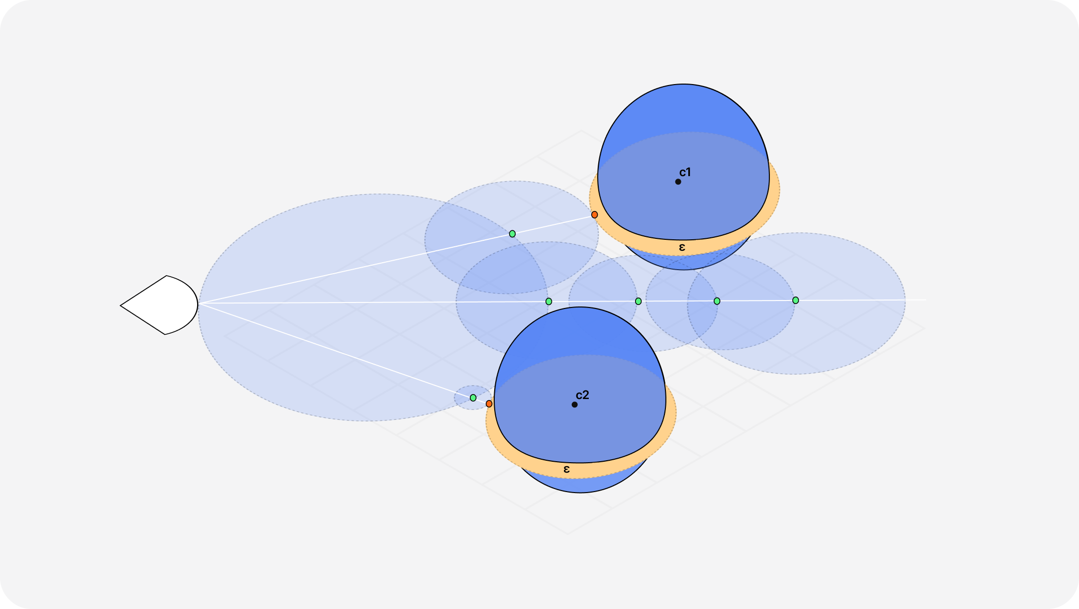
For each step, calculating and marching that resulting distance along the rays lets us approach those objects until we're close enough to consider we've "hit" the surface and can draw a pixel. The diagrams below showcase this process:

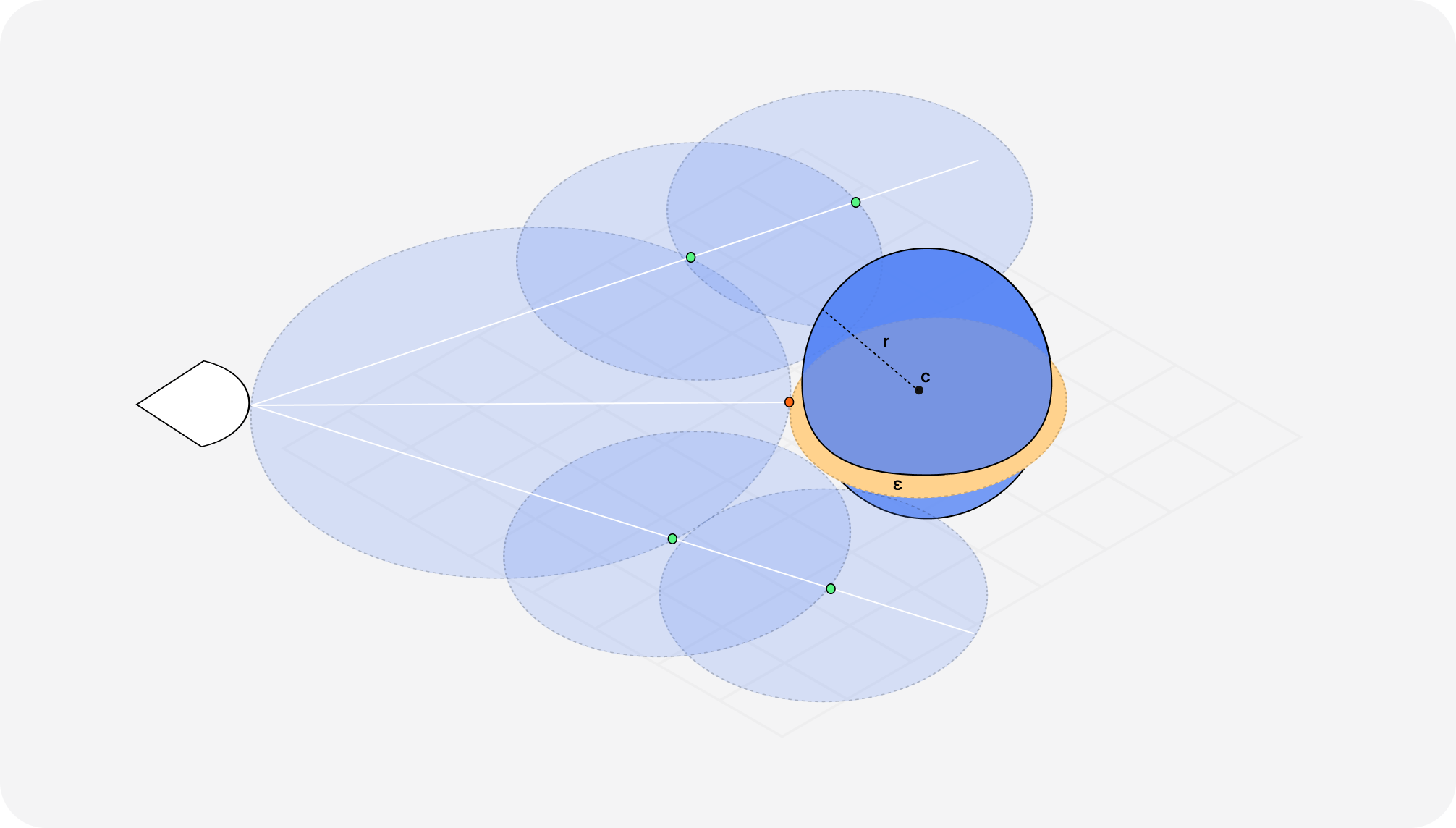
Notice how:

• each step of the raymarching (in green) goes as far as the distance to the object.
• if the distance between a point on our rays and the surface of an object is small enough (under a small value ε) we consider we have a hit (in orange).
• if the distance is not under that threshold, we continue the process over and over using our SDF until we reach the maximum amount of steps.

By using SDFs, we can define a variety of basic shapes, like spheres, boxes, or toruses that can then be combined to make more sophisticated objects (which we'll see later in this article). Each of these have a specific formula that had to be reverse-engineered from the distance of a point to its surface. For example, the SDF of a sphere is equivalent to:

1
float sdSphere(vec3 p, float radius){
2
    return length(p) - radius;
3
}

To help you understand why the SDF of a sphere is defined as such, I made the diagram below:

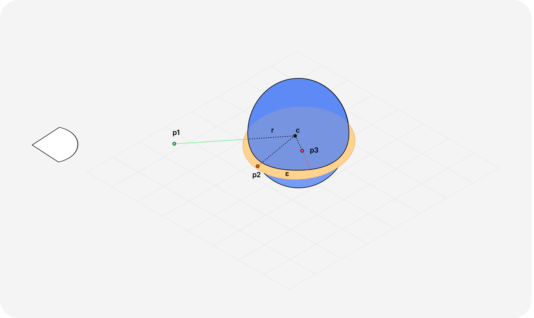
In it:

• P1 is at a distance d from the surface that is positive since the distance between P1 and the center of the sphere c is greater than the radius of the sphere r.
• P2 is very close to the surface and would be considered a hit since the distance between P2 and c is greater than r but lower than ε.
• P3 lies "within" the sphre, and technically we want our Raymarcher to never end up in such use case (at least for what is presented in this article).

This is where the Math in Raymarching resides: through the definition and the combination of SDFs, we can literally define entire worlds with math. To showcase that power however, we first need to create our first "Raymarcher" and put in code the different constructs we just introduced.

Our first Raymarched scene

This introduction to the concept of Raymarching might have left you perplexed as to how one is supposed to get started building anything with it. Lucky for us, there are many ways to render a Raymarched scene, and for this article we're going to take the perhaps most obvious approach: use a simple Three.js/React Three Fiber planeGeometry as a canvas, and paint our shader on it.

The canvas

Rendering a shader on top of a fullscreen planeGeometry is the technique I used during this Raymarching study:

• I didn't want too much time investigating more lightweight solutions.
• I still wanted to have easy access to tools like Leva.
• I was familiar with React Three Fiber's render loop and still wanted to reuse code I've written over the past two years, like uniforms, OrbitControls, mouse movements, etc.

Below is a code snippet of my canvas that served as the basis for my Raymarching work:

1
import { Canvas, useFrame, useThree } from '@react-three/fiber';
2
import { useRef, Suspense } from 'react';
3
import * as THREE from 'three';
4
import { v4 as uuidv4 } from 'uuid';
5
import vertexShader from './vertexShader.glsl';
6
import fragmentShader from './fragmentShader.glsl';
7

8
const DPR = 0.75;
9

10
const SDF = (props) => {
11
  const mesh = useRef();
12
  const { viewport } = useThree();
13

14
  const uniforms = {
15
    uTime: new THREE.Uniform(0.0),
16
    uResolution: new THREE.Uniform(new THREE.Vector2()),
17
  };
18

19
  useFrame((state) => {
20
    const { clock } = state;
21
    mesh.current.material.uniforms.uTime.value = clock.getElapsedTime();
22
    mesh.current.material.uniforms.uResolution.value = new THREE.Vector2(
23
      window.innerWidth * DPR,
24
      window.innerHeight * DPR
25
    );
26
  });
27

28
  return (
29
    <mesh ref={mesh} scale={[viewport.width, viewport.height, 1]}>
30
      <planeBufferGeometry args={[1, 1]} />
31
      <shaderMaterial
32
        key={uuidv4()}
33
        fragmentShader={fragmentShader}
34
        vertexShader={vertexShader}
35
        uniforms={uniforms}
36
        wireframe={false}
37
      />
38
    </mesh>
39
  );
40
};
41

42
const Scene = () => {
43
  return (
44
    <Canvas camera={{ position: [0, 0, 6] }} dpr={DPR}>
45
      <Suspense fallback={null}>
46
        <SDF />
47
      </Suspense>
48
    </Canvas>
49
  );
50
};
51

52
export default Scene;

I'm also passing a couple of essential uniforms to my shaderMaterial, which I advise you include as well in your own work, as they may become pretty handy to have around:

• uResolution contains the current resolution of the window.
• uTime represents the time since the scene was rendered on the screen.

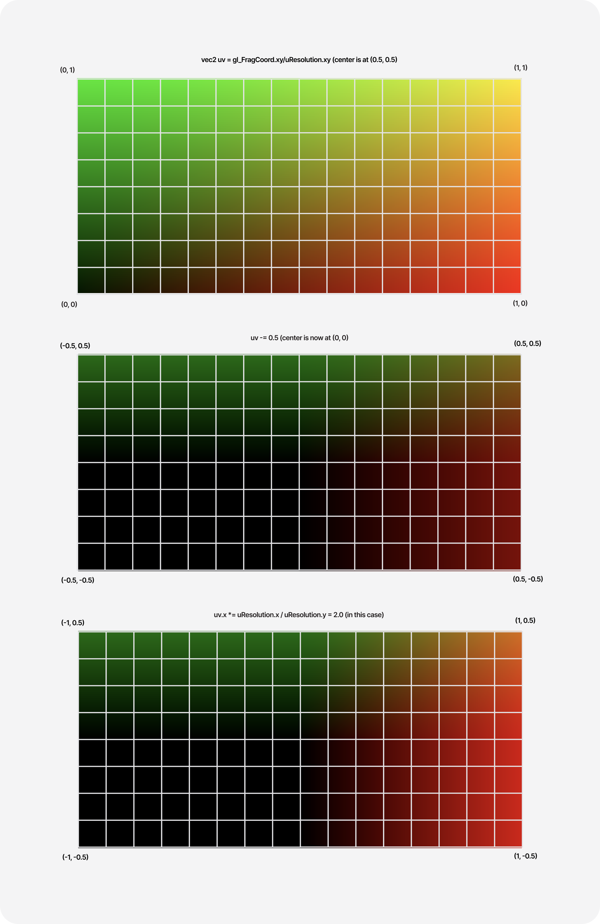
We need to do a few tweaks to our fragment shader before we can start implementing our Raymarcher:

1. Normalize our UV coordinates.
2. Shift our UV coordinates to be centered.
3. Adjust them to the current aspect ratio of the screen.

These steps allow us to have our coordinate system where the center of the screen is at the coordinates (0, 0) while preserving the appearance of our shader regardless of screen resolutions and aspect ratios (it won't appear stretched). That process may be hard to understand at first, but here's a diagram to illustrate the math involved:

Beaming rays

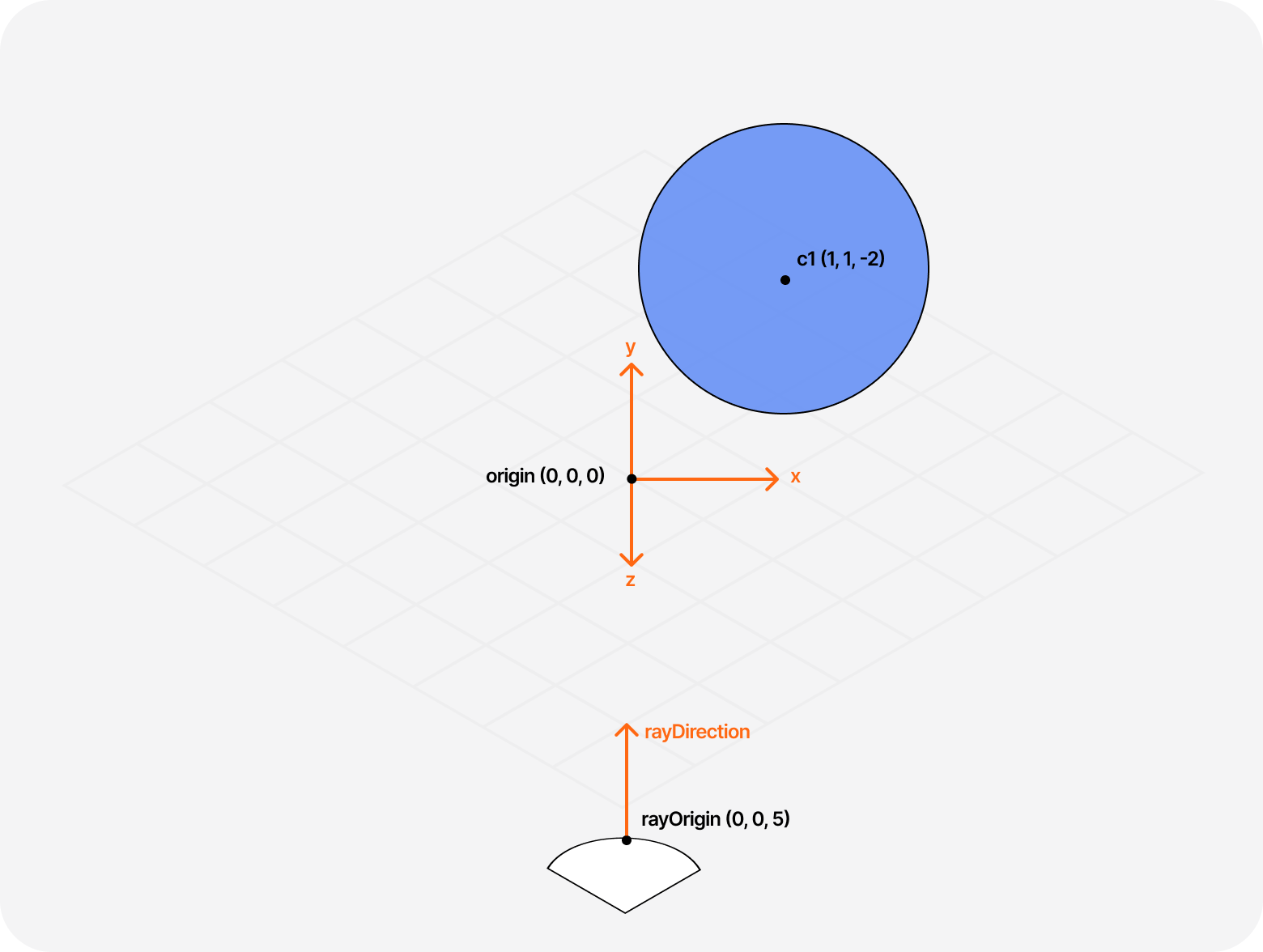
Let's implement our Raymarching algorithm step-by-step from the definition established earlier. We need:

1. A rayOrigin from where all our rays will emerge from. E.g. vec3(0, 0, 5).
2. A rayDirection equivalent to normalize(vec3(uv, -1.0)) to allow us to beam rays in every direction on the screen along the negative z-axis.
3. A raymarch function to march from the rayOrigin following the rayDirection and detect when we're close enough to a surface to draw it.
4. An SDF of any kind (we'll use a sphere) that our raymarch function will use to calculate how close it is from the surface at any given point of the raymarching loop.
5. A maximum number MAX_STEPS of steps and a surface distance SURFACE_DISTANCE from which we can safely assume we're close enough to draw a pixel.

Our raymarch function will loop for up to MAX_STEPS until we reach the step limit, in which case we'll draw nothing or hit the surface of the shape defined by our SDF.

1
#define MAX_STEPS 100
2
#define MAX_DIST 100.0
3
#define SURFACE_DIST 0.01
4

5
float scene(vec3 p) {
6
  float distance = sdSphere(p, 1.0);
7
  return distance;
8
}
9

10
float raymarch(vec3 ro, vec3 rd) {
11
  float dO = 0.0;
12
  vec3 color = vec3(0.0);
13

14
  for(int i = 0; i < MAX_STEPS; i++) {
15
    vec3 p = ro + rd * dO;
16

17
    float dS = scene(p);
18
    dO += dS;
19

20
    if(dO > MAX_DIST || dS < SURFACE_DIST) {
21
        break;
22
    }
23
  }
24
  return dO;
25
}

If we try running this code within our canvas, we should obtain the following result 👀

Adding some depth with light

We just drew a sphere with solely GLSL code 🎉. However, it looks more like a circle because our scene has no light or lighting model implemented, which means our scene doesn't have much depth. That is quite similar to the first mesh you render in Three.js using MeshBasicMaterial: the lack of shadows and reflections or diffuse makes the result look flat.

If you read my article Refraction, dispersion, and other shader light effects, we had a similar issue, and that's where we introduced the concept of diffuse light. Lucky us, we can reuse the same formula and principles from that blog post: by using the dot product of the normal of the surface and a light direction vector, we can get some simple lighting in our raymarched scene 💡.

1
float diffuse = max(dot(normal, lightDirection), 0.0);

The only issue is that we do not have an easy access to the Normal vector as we do in rasterized scenes. We need to calculate it for each "hit" we get between our rays and a surface. Luckily, Inigo Quilez already went deep into this subject, and I invite you to read his article on the subject as it will give you a better understanding of the underlying formula which we'll use throughout all the examples of this article:

1
vec3 getNormal(vec3 p) {
2
  vec2 e = vec2(.01, 0);
3

4
  vec3 n = scene(p) - vec3(
5
    scene(p-e.xyy),
6
    scene(p-e.yxy),
7
    scene(p-e.yyx));
8

9
  return normalize(n);
10
}

Applying both those formulas gives us a nicely lit raymarched scene 💡. Sprinkle on top some uTime for our light position, and we can appreciate a more dynamic composition that reacts to light in real-time:

SDF operations, complex scenes, and fractals

Using SDFs lets us render a plethora of objects in our raymarched scenes, but there's more we can do with them. In this part, we'll go through different applications of SDFs to create more complex compositions by:

• rendering multiple objects
• combining shapes to create new ones
• moving, scaling, and rotating objects

Combining SDFs

To render two objects within a raymarched scene where each object is defined through their respective SDF, we need to return a distance equivalent to the minimum of both SDFs. This is perhaps one of the technique you'll use the most throughout your own Raymarching explorations.

1
float scene(vec3 p) {
2
  float plane = p.y;
3
  float sphere = sdSphere(p, 1.0);
4

5
  float distance = min(sphere, plane);
6
  return distance;
7
}

Why is it the min?

Doing the min of two SDFs consists of uniting the two shapes in a single scene: either object could get hit by the ray, and you're essentially asking which of the two shapes is closer to a given point.

This is represented in the graph below 👇, notice how we march our rays a distance d, that is for any given point on that ray, equivalent to the distance to the closest object in the scene.

Thus, if the objects are far apart, doing the min of both SDFs will render both on the scene. If they are close enough, it will look as if they are blending into one another 🫧.

Likewise, if we were to do the max of two SDFs, we'd render the intersection of both objects: you'd be looking for when your ray is inside both SDFs. That one is my favorite operator, as it allows us to build very sophisticated shapes using techniques akin to CSG (Constructive Solid Geometries).

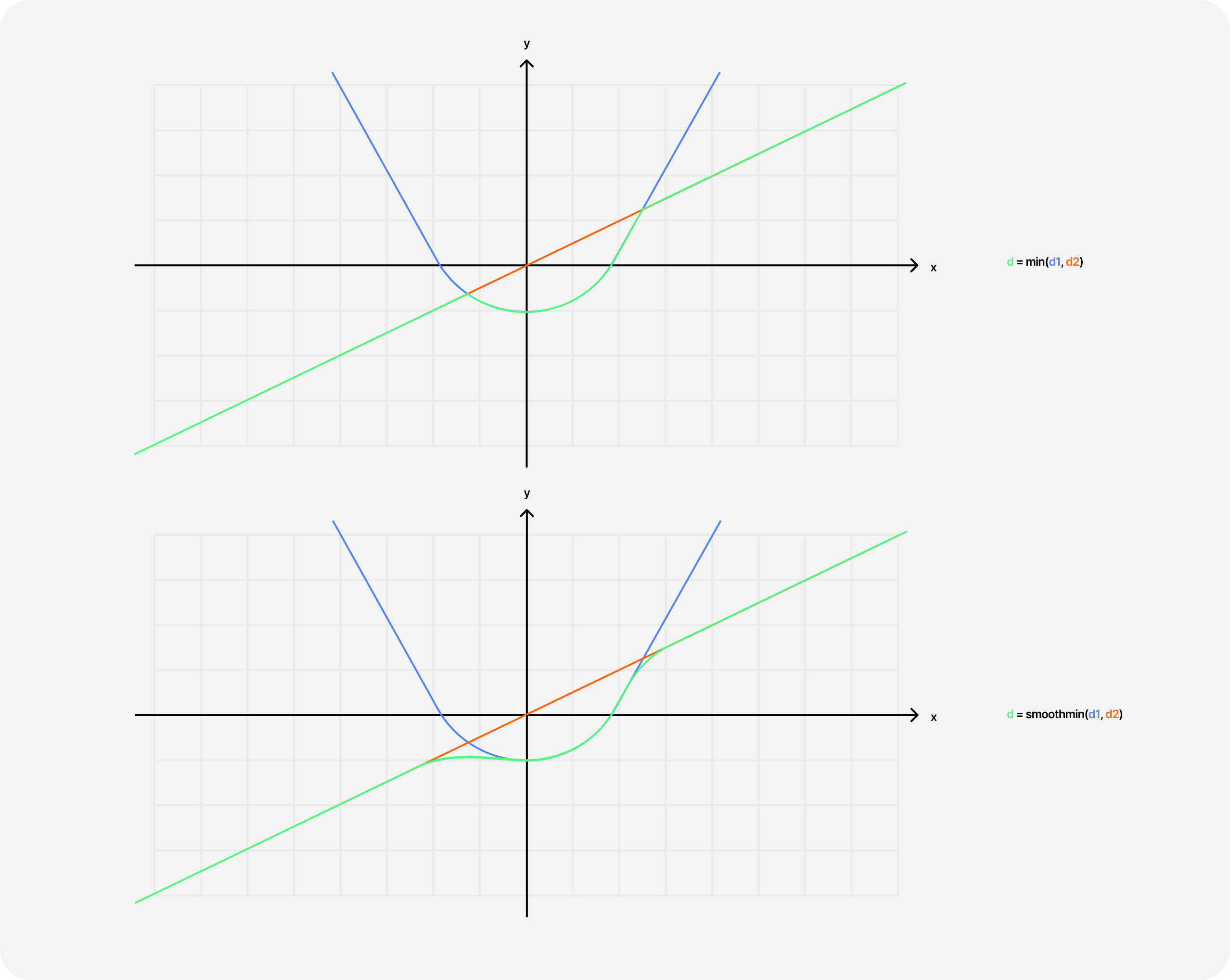
However, an issue that is particularly visible in the examples above is that these operators do not yield very smooth unions and intersections. That is due to discontinued derivatives of the surfaces, a.k.a. the slopes. At a single point we have:

• one surface that has a downward slope (negative derivative)
• another surface that has a upward slope (positive derivative)

We can use a pinch of math to obtain a smooth minimum/maximum. Once again, Inigo Quilez wrote on the subject pretty extensively, and his polynomial smoothmin variant became the standard in many Shadertoy scenes. This video from The Art of Code also goes into more details but with a more visual approach on how to get to the formula step-by-step.

1
float smoothmin(float a, float b, float k) {
2
  float h = clamp(0.5 + 0.5 * (b-a)/k, 0.0, 1.0);
3
  return mix(b, a, h) - k * h * (1.0 - h);
4
}

Thanks to this smoothmin function, we can not only get prettier unions, but we can also have objects act more like liquids or more organic when moving and blending together. That's something that is quite difficult to do in a rasterized scene and would require a lot of vertices, but it only requires a few lines of GLSL to obtain a great result with Raymarching!

The scene below is an example of smooth minimum applied to three spheres alongside some Perlin noise, akin to the one I made for this showcase.

Moving, rotating, and scaling

While the union and intersection of SDFs may be straightforward to picture in one's mind, operations such as translations, rotations, and scale can feel a bit less intuitive, especially when having only dealt with rasterized scenes in the past.

To me, to position a sphere in a raymarched scene at a given set of coordinates, it first made more sense to render the SDF, pick it up, and move it to the desired position, which, unfortunately for this intuition, is wrong. In the world of Raymarching, you'd need to move the sampling point to the opposite direction you wish to place your SDF object. A simple way to visualize this is to:

• Imagine yourself as a point in a raymarched scene containing a sphere.
• If you step two steps to the right, your sphere will appear to you two steps further to the left.

1
float scene(vec3 p) {
2
  float plane = p.y + 1.0;
3
  float sphere = sdSphere(p - vec3(0.0, 1.0, 0.0), 1.0);
4

5
  float distance = min(sphere, plane);
6
  return distance;
7
}

Rotating consists of the same way of thinking:

• We don't rotate the SDF itself
• We apply the rotation on the sampling point instead

1
float scene(vec3 p) {
2
  vec3 p1 = rotate(p, vec3(0.0, 1.0, 0.0), 3.14 * 2.0);
3
  float distance = sdSphere(p1, 1.0);
4

5
  return distance;
6
}

Scaling is even weirder. To scale, you need to multiply your sampling point by a factor:

• Multiplying by two will make the resulting shape half the size
• Multiplying by 0.5 will make the shape twice as big

However, by multiplying our sampling point, we mess a bit with our raymarcher and may accidentally have it step inside our object. To work around this issue, we have to decrease our step size (i.e. the distance returned by the SDF) by the same factor we're scaling our shape of

1
float scene(vec3 p) {
2
  float scale = 2.0;
3
  vec3 p1 = p * scale;
4

5
  float sphere = sdSphere(p1, 1.5);
6
  float distance = sphere / scale;
7

8
  return distance;
9
}

Combining all those operations and transformations and adding our utime uniform to the mix can yield gorgeous results. You can see one such beautifully executed raymarched scene that uses those operations on Richard Mattka's portfolio, which @Akella reproduced in one of his streams.

I give you my own simplified implementation of it below, also featured on my React Three Fiber showcase website, which leverages all the building blocks of Raymarching featured in this article so far:

Scaling to infinity

One trippy aspect of Raymarching that really blew my mind early on is the ability to render infinite-looking scenes with very little code. You can achieve that by putting together lots of SDFs, positioning them programmatically, moving your camera, or increasing the maximum number of steps to render further in space. However, the more SDFs we use, the slower our scene gets.

If you've tried to do the same in a classic rasterized scene, you have faced the same issues and worked around them using mesh instances instead of rendering discreet meshes. Luckily, Raymarching lets us use a similar principle: reusing a single SDF to add as many objects as desired onto our scene.

1
vec3 repeat(vec3 p, float c) {
2
    return mod(p,c) - 0.5 * c; // (0.5 *c centers the tiling around the origin)
3
}

The function above is what makes this possible:

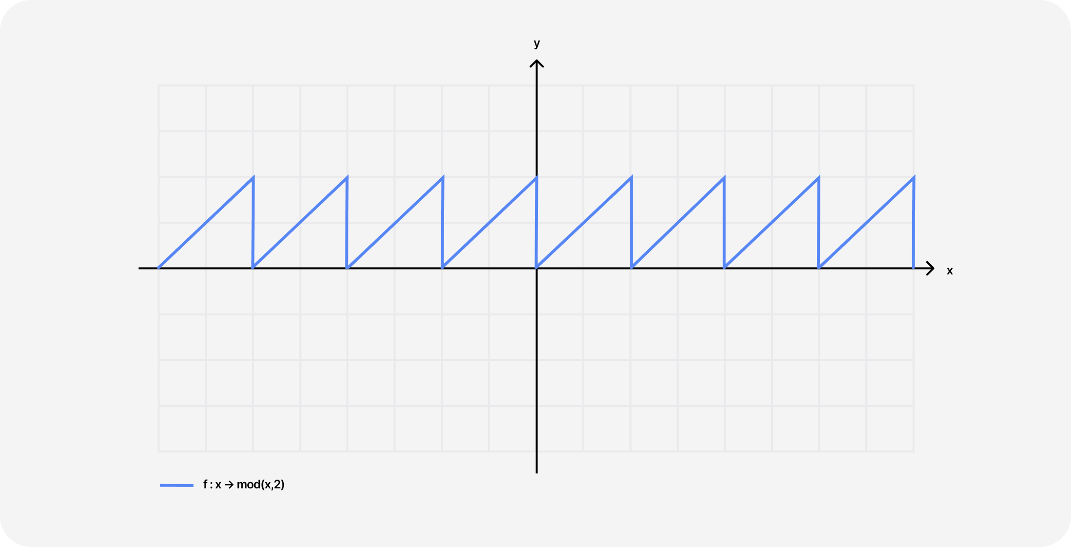
• Using the mod function (modulo) on the sampling point p lets us take a chunk of space defined by the second argument and tile it infinitely in all directions (see diagram below showcasing the mod function but applied only to a single dimension).
• Then, "instantiate" many objects from a single SDF for each tile, giving the illusion of infinite shapes stretching to infinity.

The demo scene below showcases how you can include the repeat function with any SDF to create infinite instances of an object in every direction in space:

Notice that if the second argument of the modulo function is low, the objects will appear closer to one another (more frequent repetitions). If higher, they will appear further apart.

While being able to render scenes that stretch to infinity is impressive, the mod function can also have an incredible effect in a more "limited" way: to create fractals.

That's what Inigo Quilez explores in his article about Menger Fractals which are nothing more than "iterated intersection of a cross and a box SDF" that solely relies on the operations we've seen in this part:

• Render a simple box using its SDF.

1
float sdBox(vec3 p, vec3 b) {
2
  vec3 q = abs(p) - b;
3
  return length(max(q, 0.0)) + min(max(q.x, max(q.y, q.z)), 0.0);
4
}
5

6
float scene(vec3 p) {
7
  float d = sdBox(p,vec3(6.0));
8

9
  return d;
10
}

• Render an infinite cross SDF, which is the union of 3 boxes.
• Intersect them to obtain a box with square holes at the center of each phase using the max operator.

1
float sdBox(vec3 p, vec3 b) {
2
  vec3 q = abs(p) - b;
3
  return length(max(q, 0.0)) + min(max(q.x, max(q.y, q.z)), 0.0);
4
}
5

6
// The SDF of this cross is 3 box stretched to infinity along all 3 axis
7
float sdCross( in vec3 p ) {
8
  float da = sdBox(p.xyz,vec3(inf,1.0,1.0));
9
  float db = sdBox(p.yzx,vec3(1.0,inf,1.0));
10
  float dc = sdBox(p.zxy,vec3(1.0,1.0,inf));
11
  return min(da,min(db,dc));
12
}
13

14
float scene(vec3 p) {
15
  float d = sdBox(p,vec3(6.0));
16
  float c = sdCross(p);
17

18
  float distance = max(d,c);
19
  return distance;
20
}

By doing these operations in a loop, and for each iteration, making our combined SDF smaller by scaling down and increasing the number of repetitions, the resulting SDF can output some intricate objects that can display repeating patterns that could theoretically go on forever if we wanted to. Hence, this falls into the category of fractals.

The demo below showcases the Menger fractal implementation from Inigo, using the building blocks we laid out in this article with the inclusion of soft shadows, which really shine (no pun intended) for this specific use case.

Building Worlds with Raymarching and noise derivatives

We've finally reached the part focusing on the reason I wanted to write this blog post in the first place ✨. Now that we've warmed up and got familiar with the building blocks of Raymarching, we can explore the beautiful art of painting landscapes with those same techniques.

If you spend some time searching on Shadertoy, those raymarched landscapes can feel both breathtaking when looking at the results they yield and quite intimidating at the same time when looking at the code displayed on the right-hand side of the website. That is why I spent a big deal of time analyzing a couple of those landscapes by trying to find the repetitive patterns used by the authors and breaking them down for you into more digestible bits.

Composing noise with Fractal Brownian Motion

You've probably played quite a bit with noise in your own shader work and are familiar with the ability of the different types to generate more organic patterns.

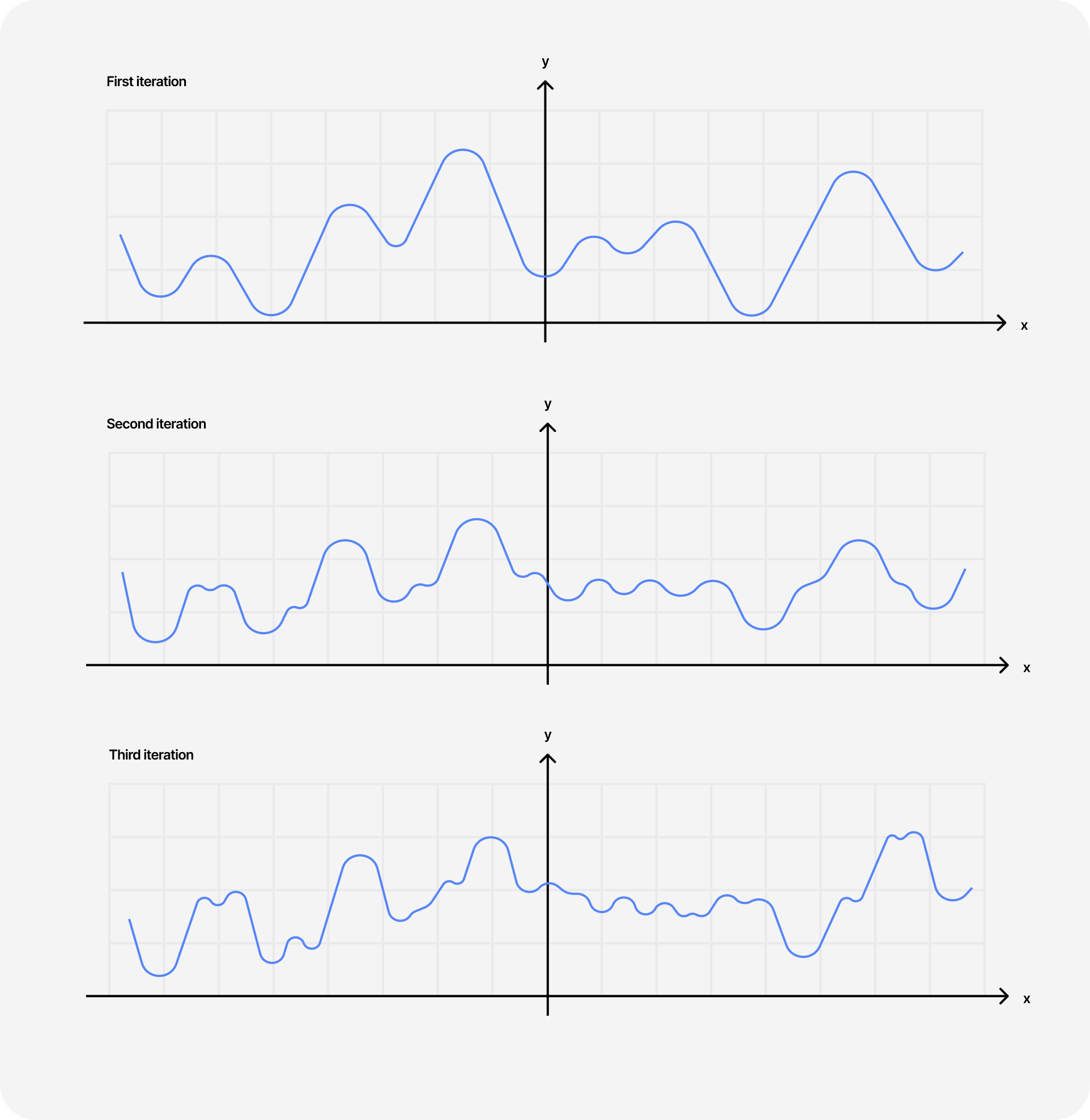
In that blog post, I also briefly mention the concept of Fractal Brownian Motion: a method to compose noises and obtain a more granular resulting noise featuring more fine details:

• The final detailed noise builds itself in a loop.
• We start with a simple noise with a given amplitude and frequency for the first iteration.
• Then, for each iteration, we apply the same noise but decrease the amplitude and increase the frequency (and add some transformation if we want to), thus creating sharper details but with less influence on the overall scene.

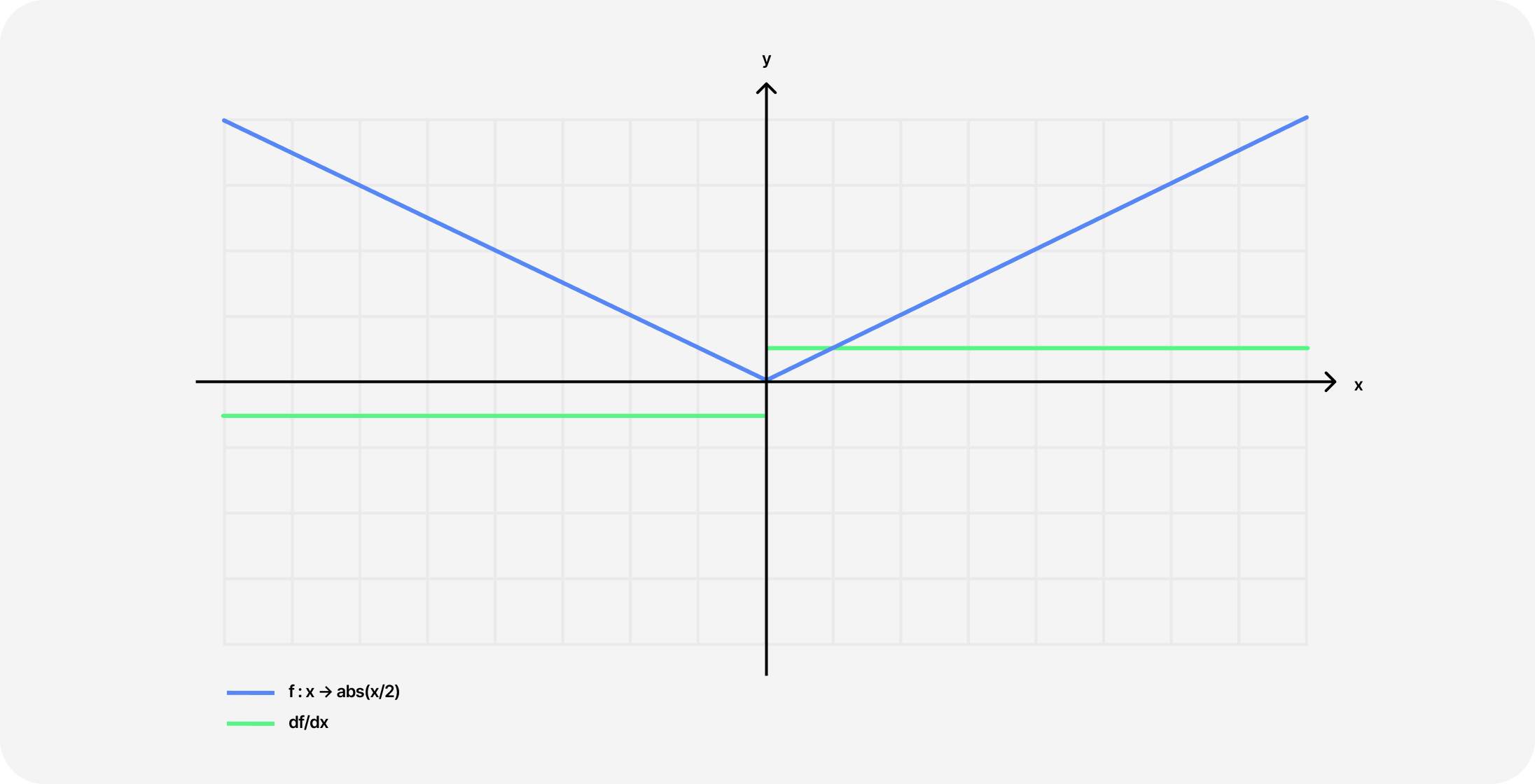
We can visualize this in 2D by looking at a simple curve. Each iteration is called an Octave, and the higher we go in terms of octaves, the sharper and better looking our noise will be:

Applying that type of noise to the SDF of a plane, like in the code snippet below, can yield some very sharp-looking mountainous landscapes stretching to infinity.

1
// importing perlin noise from glsl-noise through glslify
2
#pragma glslify: cnoise = require(glsl-noise/classic/2d)
3

4
#define PI 3.14159265359
5

6
mat2 rotate2D(float a) {
7
  float sa = sin(a);
8
  float ca = cos(a);
9
  return mat2(ca, -sa, sa, ca);
10
}
11

12
float fbm(vec2 p) {
13
  float res = 0.0;
14
  float amp = 0.8;
15
  float freq = 1.5;
16

17
  for(int i = 0; i < 12; i++) {
18
    res += amp * cnoise(p * 0.8);
19
    amp *= 0.5;
20
    freq *= 1.05;
21
    p = p * freq * rotate2D(PI / 4.0);
22
  }
23
  return res;
24
}
25

26
float scene(vec3 p) {
27
  float distance = 0.0;
28
  distance += fbm(p.xz * 0.3);
29
  distance += p.y + 2.0;
30

31
  return distance;
32
}

Add to that the diffuse lighting model we looked at in the earlier parts of this article and some soft shadows, and you can get a beautiful raymarched landscape with just a few lines of GLSL. Those are the techniques I used to build my very first raymarched terrain, and I was quite satisfied with the result. Also, look at how the shadows update in real time as we move the position of the light 🤤.

Maxime@MaximeHeckel

You can create entire procedurally generated worlds with shaders with a couple of well-placed math formulas! From the sharpness of the terrain, the light, the fog, and the shadows of those mountains: it's all GLSL (don't run this on your phone pls) https://t.co/hBVew9w90O https://t.co/jl1vk9yPWQ

2:40 AM - Jul 13, 2023

7176

However, I quickly realized that:

1. I needed my FBM loop to reach high octaves for a sharp looking result. That caused the frame rate to drop significantly, as the higher the octaves for my FBM, the higher the complexity of my raymarcher was (nested loops). This scene was pulling a lot of juice from my laptop and even worse at higher resolutions!
2. Despite using Perlin noise as the base for my FBM, the resulting landscape was just an endless series of mountains. Each looked distinct and unique from its neighbor, but the overall result looked repetitive.

Noise derivatives

By studying Inigo's own 3D landscape creations, I noticed that in many of them, he was using a tweaked Fractal Brownian Motion to generate his terrains through the use of noise derivatives.

In his blog posts on the topic, he presents this technique as an updated version of FBM to generate realistic-looking noise patterns. This technique is, at first glance, a little bit more complicated to explain concisely and also involves a little bit more math than most people might be comfortable with, but here's my own attempt at highlighting its key features:

• It relies on sampling a grayscaled noise texture (we'll get to that in a bit) at various points, i.e. looking at the color value stored at a given location, and interpolating between them.
• Instead of relying on those "noise values", we're using the derivative between the sampled points representing the steepness or rate of change.

We thus end up with more "data" about the physical properties of our terrain: the higher derivatives correspond to steeper regions of our landscapes, while lower values will result in flat plateaux or downward slopes, resulting in better-looking, more detailed terrains. The GLSL code for that function looks like this 👇

1
// Noise texture passed as a uniform
2
uniform sampler2D uTexture;
3

4
vec3 noised(vec2 x) {
5
  vec2 p = floor(x);
6
  vec2 f = fract(x);
7
  vec2 u = f * f* (3.0 - 2.0 * f);
8

9
  float a = textureLod(uTexture, (p+vec2(.0,.0)) /256.,0.).x;
10
  float b = textureLod(uTexture, (p+vec2(1.0,.0)) /256.,0.).x;
11
  float c = textureLod(uTexture, (p+vec2(.0,1.0)) /256.,0.).x;
12
  float d = textureLod(uTexture, (p+vec2(1.0,1.0)) /256.,0.).x;
13

14
  float noiseValue = a + (b - a) * u.x + (c - a) *
15
    u.y + (a - b - c + d) * u.x * u.y;
16
  vec2 noiseDerivative = 6.0 * f * (1.0 - f) * (vec2(b - a, c - a) +
17
    (a - b - c + d) * u.yx);
18

19
  return vec3(noiseValue, noiseDerivative);
20
}

From these noise derivatives, we can generate the terrain in a similar fashion to the FBM method. For each iteration:

• We call our noised function for our sample point.
• Accumulate the derivatives, which will accentuate the features of the terrain as we go through the iterations of our loop.
• Adjust the height a of our terrain based on the value of the noise.
• Reduce and flip the sign of the scaling factor b. That will result in each subsequent iteration having less effect on the global aspect of the terrain while also alternating between increases and decreases in the overall height of our terrain.
• Transform the sampling point for the next loop by multiplying it by a rotation matrix (which results in a slight rotation for the following iteration) and scaling it down.

1
float terrain(vec2 p){
2
  vec2 p1 = p * 0.06;
3
  float a = 0.0;
4
  float b = 2.5;
5
  vec2 d = vec2(0.0);
6
  float scl = 2.75;
7

8
  for(int i = 0; i < 8; i++ ) {
9
    vec3 n = noised(p1);
10
    d += n.yz;
11
    a += b * n.x / (dot(d,d) + 1.0);
12
    b *= -0.4;
13
    a *= .85;
14
    p1 = m * p1 * scl;
15
  }
16

17
  return a * 3.0;
18
}

The screenshot below showcases the terrain yielded at each octave (i.e. each iteration of our FBM loop) from 2 to 7:

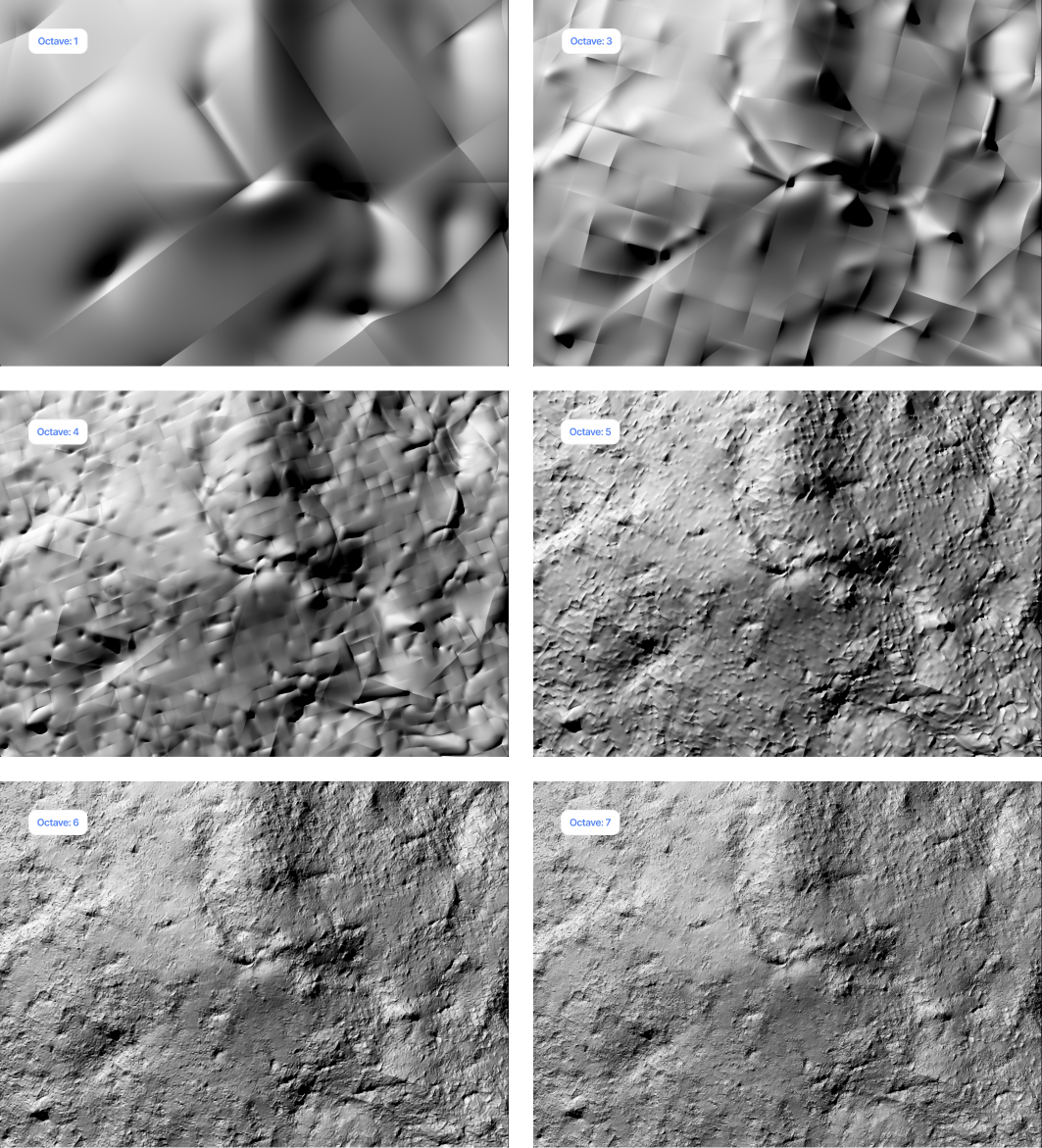
Applying this technique on top of everything we've learned through this article gives us a magnificent landscape that is entirely tweakable, more detailed, and less repetitive than its standard FBM counterpart. I'll let you play with the scale factors, noise weight, and height in the demo below so you can experiment with more diverse terrains 👀.

Sky, fog, and Martian landscape

Generating the terrain is not all there is when building landscapes with Raymarching. One of the foremost things I like to add is fog: the further in the distance an element of my landscape is, the more faded and enveloped in mist it should appear. This adds a layer of realism to the scene and can also help you color it!

Once again, we can use some math and physics principles to create such an effect. Using Beer's law which states that the intensity of light passing through a medium is exponentially related to the distance it travels we can get a realistic fog effect:

I = I0​ * exp(−α * d) where α is the absorption or attenuation coefficient describing how "thick" or "dense" the medium is.

That's the math that Inigo uses as the base for his own fog implementation that is a little bit more elaborated and is also featured in most of his own creations.

1
// This fog is presented in Inigo Quilez's article
2
// It's a version of the fog function that keeps the "fog" at the
3
// bottom of the scene, and doesn't let it go above the horizon/mountains
4
vec3 fog(vec3 ro, vec3 rd, vec3 col, float d){
5
  vec3 pos = ro + rd * d;
6
  float sunAmount = max(dot(rd, lightPosition), 0.0);
7

8
  float b = 1.3;
9
  // Applying exponential decay to fog based on distance
10
  float fogAmount = 0.2 * exp(-ro.y * b) * (1.0 - exp(-d * rd.y * b)) / rd.y;
11
  vec3 fogColor = mix(vec3(0.5,0.2,0.15), vec3(1.1,0.6,0.45), pow(sunAmount,2.0));
12

13
  return mix(col, fogColor, clamp(fogAmount,0.0,1.0));
14
}

When it comes to adding a background color for our sky, it's really straightforward: whatever was not hit by the raymarching loop is our sky and thus can be colored in any way we want!

1
vec3 lightPosition = vec3(-1.0, 0.0, 0.5);
2

3
void main(){
4
  vec2 uv = gl_FragCoord.xy/uResolution.xy;
5
  uv -= 0.5;
6
  uv.x *= uResolution.x / uResolution.y;
7

8
  vec3 color = vec3(0.0);
9
  vec3 ro = vec3(0.0, 18.0, 5.0);
10
  vec3 rd = normalize(vec3(uv, 1.0));
11

12
  float d = raymarch(ro,rd);
13
  vec3 p = ro + rd * d;
14

15
  vec3 lightDirection = normalize(lightPosition-p);
16

17
  if (d<MAX_DIST){
18
    vec3 normal = getNormal(p);
19

20
    float amb = clamp(0.5 + 0.5 * normal.y, 0.0, 1.0);
21
    float diffuse = clamp(dot(normal, lightDirection), 0.0, 1.0);
22
    float shadow = softShadows(p, lightDirection, 0.1, 3.0, 64.0);
23

24
    color = vec3(1.0) * diffuse * shadow;
25
    // apply fog to raymarched landscape
26
    color = fog(ro, rd, color, d);
27
  } else {
28
    // color the background of the scene
29
    color = vec3(0.5,0.6,0.7);
30
  }
31

32
  gl_FragColor = vec4(color, 1.0);
33
}

From there, it's up to you to get creative and play with more effects or add more details to your landscapes. I haven't had the time yet to generate a lot of those or explore how to add more details such as clouds or trees. That's next on my list though!

In case you need an example to get you started, here's a demo featuring the Martian landscape I showcased on Twitter in early August inspired by the work of @stormoid.

Maxime@MaximeHeckel

A look at some of my recent shader Raymarching work 🧪 I learned how to use noise derivatives to create better procedural terrains Combined with fog and light scattering you can achieve some gorgeous results like this beautiful Martian landscape https://t.co/5vGVFF6QgI https://t.co/UCdpr68VbK

Maxime@MaximeHeckel

You can create entire procedurally generated worlds with shaders with a couple of well-placed math formulas! From the sharpness of the terrain, the light, the fog, and the shadows of those mountains: it's all GLSL (don't run this on your phone pls) https://t.co/hBVew9w90O https://t.co/jl1vk9yPWQ

2:40 AM - Jul 13, 2023

7176

3:14 PM - Jul 31, 2023

2128

It features:

• Our good ol' Raymarcher we built in the first part of this article.
• An application of noise derivatives
• Soft shadows
• Fog
• @Stormoid's atmospherical scattering function that creates this "planetary glow" that's also based on a flavor of exponential decay (like our fog).

Final thoughts

I find those raymarched landscapes really fascinating. Through the brevity of the code, and the very realistic terrains that stretches to infinity it outputs, it makes creating large unique worlds almost trivial, which reminded me a lot of the empty, unfathomably big worlds featured in one of Jacob Geller's videos on Video Games that don't fake space.

On top of all that, the file containing the code bringing those worlds to life only weighs a couple of kilobytes, ~5kB the last time I checked for the Martian landscape excluding the texture which is itself 10x bigger already but it can technically be replaced by a hash function so I'm not counting it in. Even just taking a screenshot of a single frame of the landscape can be close to 100x heavier. I don't know about you but this makes me think a lot 😄, perhaps a bit too much, hence why I really liked working on those scenes.

All of that is made possible by simply stitching a couple of clever math together alongside some simple physics principles, which reminds me of this quote from Zach Lieberman:

zach lieberman@zachlieberman

every image I make is a snapshot of math

10:10 AM - Apr 1, 2022

6110

I think this fits well for Raymarching as a whole and also to conclude this (long) article, which I hope you enjoyed.

I'm not 100% done with Raymarching yet though (and will probably never be). If anything, this is just the tip of the iceberg. I recently got into Volumetric rendering, the method behind rendering smoke and clouds, which is kind of a spin-off of Raymarching, that I find really fun to build with. That, however, will be a topic for another time 😄.