Lighting That Feels Just Right
In The Gap, Ira Glass talks about the frustration of your output falling short of what you originally envisioned when learning a new skill. You have a clear picture in your mind about what you want, but you can't quite pull it off just yet. That feeling, I'm a bit too familiar with it, spending countless hours staring at my own shader work without being able to pinpoint why it feels off. So I started comparing my work with that of other creative devs out there and realized that more often than not, that gap was something as "simple" as lighting.
Just like in real life, the way light interacts with surfaces and materials is key to making a scene look and feel a certain way. In my work, however, it was missing something: my shadows felt harsh and my surfaces disconnected, lacking color bleeding or color contribution from the sky, to name a few.
This led me to explore more advanced techniques to solve this, all the way to path tracing 1 which, despite being too intensive to use in my projects, showed me what real Global Illumination looked like and what it could bring to my scenes: illuminated white walls reflecting light into shadowed areas, or colored objects tinting their surroundings. It was the lighting I had been missing all along. So I started exploring cheaper ways to approximate that same indirect lighting in real time.
As you may guess, this sent me on yet another side quest, which became the catalyst for this article. I spent several weeks teaching myself the inner workings of GI and building demos each step of the way. I started with Screen-Space Global Illumination, then explored a more practical and flexible probe-based approach, before finally combining the results with reflections, volumetric lighting, and atmospheric scattering contributions, all topics I've dived into earlier in my journey. I’m excited to show you the visuals I achieved, and even more so, to share how I got there.
First, let’s revisit the lighting model we’ve used many times throughout my articles: the Blinn-Phong lighting model 2. It’s easy to understand and very handy for giving materials simple diffuse shading and highlights with just a few lines of code.
Intuitively, it works as follows:
- When the normal of a point on a surface is perfectly aligned with the light direction, that point receives the most light.
- As the angle between the normal and the light direction increases, the point receives less and less light.
- Finally, once the normal is perpendicular to, or further from, the light direction, the point receives no light.
That behavior is what’s represented by the diffuse lighting term max(dot(normal, lightDirection), 0.0). However, this only accounts for the direct light, which means:
- Surfaces facing away from the light are completely dark, and vice versa, the more toward the light your surface is facing, the brighter it will be.
- Only the direct light matters. A brightly lit surface contributes no lighting at all to the objects or scene around it.
Adding ambient lighting to fake some indirect lighting and brighten up those darker regions is a quick solution, but it doesn’t account for where the light comes from, which surfaces it reaches, or the colors that are picked up along the way. That's just not how light works.
What I learned through path tracing is that light keeps traveling after it hits a surface; it bounces, thus ending up illuminating surfaces it did not reach directly.
A lit white wall can contribute light to the back of objects that the light didn't hit, or an orange sphere can leave an orange tint on the floor it touches 3. These side effects can fit under the umbrella of indirect lighting and are what we’ll be computing, but I should rather say approximate, throughout this article when exploring cheaper ways to achieve Global Illumination.
Below is an example of how much indirect light, in this case implemented through the methods we'll see, can change a given scene:
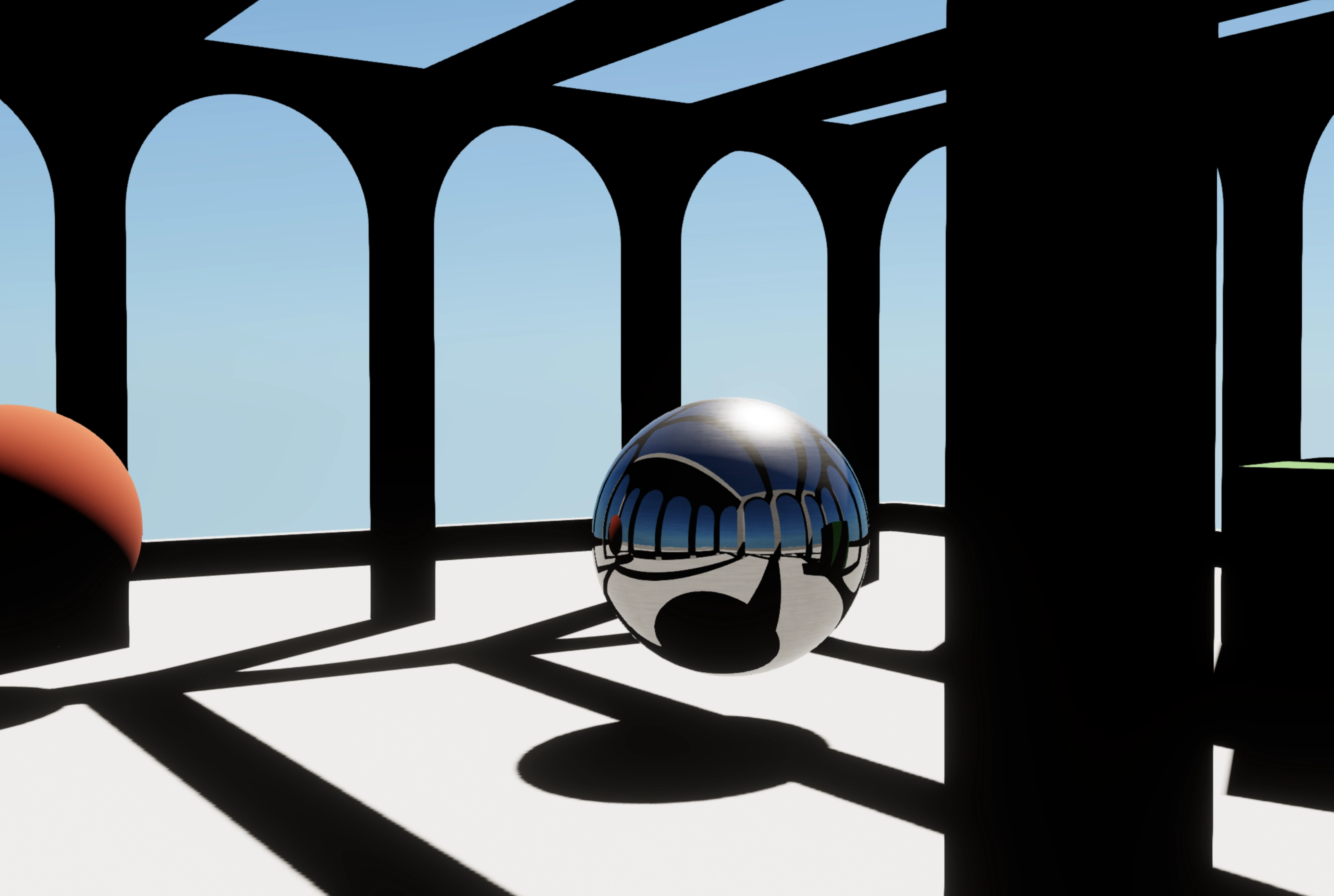
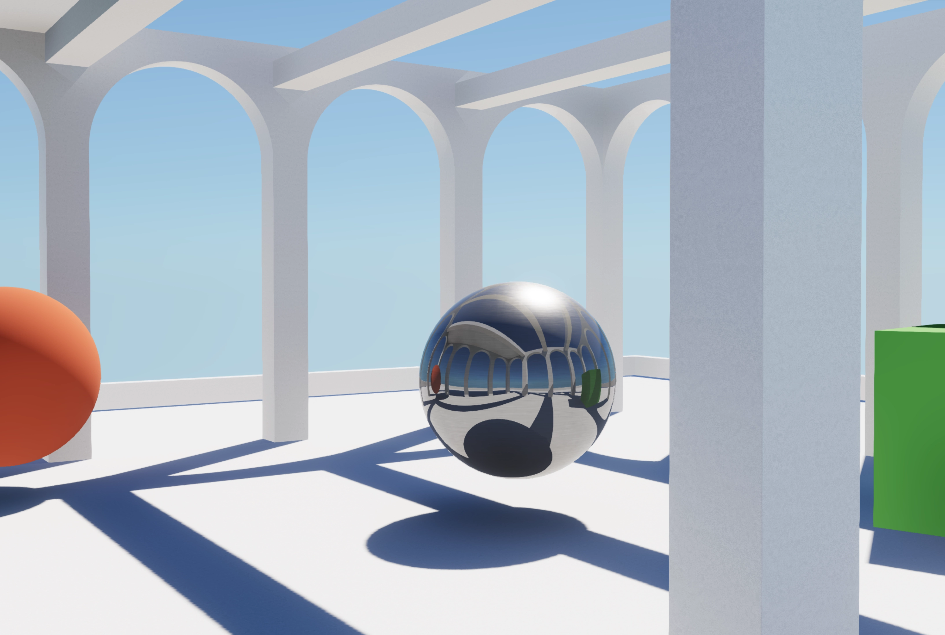
Having worked with Screen Space post-processing effects before through Volumetric Lighting or Atmospheric Scattering 4, I wanted to approach GI from familiar grounds. My goal was to see whether leveraging pixels from surfaces visible on screen at any given frame was enough to compute pleasing yet convincing indirect light.
Of course, the color of the pixel is not enough for us to deduce where the surfaces are and how they relate to each other in space, we first have to reconstruct their position in 3D space and from there march rays through the scene to look for those surfaces and estimate the light they contribute back. In our Volumetric Lighting work, we had to reconstruct a surface’s position to know when to stop marching a ray from the camera 5. In this case, however, they give us a starting point for our raymarching on the surface itself.
At a high level, this process works as follows, for any given pixel of the frame:
- We reconstruct the position of the surface
- We use its normal to orient a hemisphere and sample directions with it
- We raymarch from the point on the surface along those directions
- We compare each ray’s depth with the scene’s depth to find another surface
- We sample that surface’s color to estimate its lighting contribution
- We average the samples and apply the receiving light/color/albedo to estimate the indirect lighting for said position. The albedo, in this case, is the receiving surface’s base color.
I detailed the process step-by-step, visually, in the interactive diagram below. It’s a simplified version of what actually happens, but it will give you a good idea of the mechanisms at play here:
Pixels to surfaces
For this, we will leverage the depth and normal map of our frame. Together, these 2 textures give us the information we need to know where to start our rays and orient them. To do so, we’ll:
- Create a
scenePassthat renders our scene into textures that we’ll later access from our post-processing effect. Using themrtTSL function, we’re capturing the rendered colors, normals, and albedo, or “base color”.
1// sample: 0 disables multisample antialiasing for this pass, simplifying depth sampling.2const scenePass = pass(scene, camera, { samples: 0 });34scenePass.setMRT(5mrt({6output,7normal: normalWorld,8albedo: materialColor,9}),10);1112const sceneColor = scenePass.getTextureNode('output');13const depth = scenePass.getTextureNode('depth');14const normals = scenePass.getTextureNode('normal');15const albedo = scenePass.getTextureNode('albedo');
- Using the depth of the scene, recover the position relative to the camera and transform that position into world space.
1const viewPosition = getViewPosition(2uv(),3depth.r,4uniform(camera.projectionMatrixInverse),5);67const worldPosition = uniform(camera.matrixWorld).mul(8vec4(viewPosition, 1),9).xyz;
With this, we can get the 3D position of the surface visible at each pixel of our rendered frame, and paired with our normal data, we also know which way said surface faces. These coordinates and surface orientation will serve as the starting point for our raymarching process, from which we’ll estimate indirect light contributions.
Hemisphere and rays
A surface can receive light from many directions, so we can’t just trace a single ray and hope to get a reliable estimate of its indirect lighting. Instead, we’ll trace several rays across a hemisphere, in the examples below, 8 per pixel, to find other surfaces and estimate the light they contribute.
For our opaque surfaces, we’ll sample directions within the hemisphere above each surface, oriented along its normal. We’ll use a cosine-weighted hemisphere to put more weight on directions closer to the surface’s normal rather than those grazing the surface.
The code snippet below establishes this distribution of directions:
Defining our cosine-weighted hemisphere
1let n = normalize(surfaceWorldNormal);23// Build a local coordinate frame around the surface normal.4var axis = vec3f(0.0, 0.0, 1.0);56if (abs(n.z) > 0.999) {7axis = vec3f(0.0, 1.0, 0.0);8}910let tangent = normalize(cross(axis, n));11let bitangent = cross(n, tangent);1213let pixel = vec2u(screenUV * samplingResolution);1415// Generate eight cosine-weighted hemisphere directions.16for (var i = 0u; i < 8u; i++) {17let random = hash23(18vec3f(vec2f(pixel), f32(i + 16u))19);2021// Give each ray its own interval to reduce clumping.22let u1 = (f32(i) + random.x) / 8.0;23let u2 = random.y;2425// Sample a disk, then lift the sample onto a hemisphere.26let radius = sqrt(u1);27let phi = 6.28318530718 * u2;2829// Express the sampled direction in world space.30let direction =31tangent * (radius * cos(phi))32+ bitangent * (radius * sin(phi))33+ n * sqrt(1.0 - u1);3435// WE WILL TRACE RAYS FROM HERE36}
It may seem obtuse at first, but it can luckily be broken down into very simple steps:
From there, we can use those newly defined directions to trace our rays. Each of the 8 rays starts at the surface position we reconstructed earlier:
1let direction = normalize(rayDirection);2let origin = surfaceWorldPosition + normalize(surfaceWorldNormal) * 0.05;
These will each help us find other visible surfaces and sample the corresponding rendered color, giving us an estimate of the light coming from that direction. For this process we will:
- Advance along the ray in small step increments in view space, projecting each step onto the screen
1let originView = viewMatrix * vec4f(origin, 1.0);2let directionView = viewMatrix * vec4f(direction, 0.0);34let size = vec2i(textureDimensions(depthMap));5let stepSize = maxDistance / f32(stepCount);67var previousDelta = -1.0;89for (var i = 0u; i < stepCount; i++) {10let distance = (f32(i) + marchOffset) * stepSize;11let rayViewPosition = originView + directionView * distance;1213// Stop if the ray reaches the camera's near plane.14if (rayViewPosition.z >= -nearPlane) {15break;16}1718// Project the position into clip space, then screen UVs.19let clip = projection * rayViewPosition;20let ndc = clip.xy / clip.w;21let sampleUV = vec2f(22ndc.x * 0.5 + 0.5,230.5 - ndc.y * 0.524);2526// Stop when the ray leaves the screen.27if (any(sampleUV < vec2f(0.0)) ||28any(sampleUV >= vec2f(1.0))) {29break;30}3132// Insert the depth comparison below here.33}3435// No intersection found.36return vec3f(0.0);
- Compare the ray’s depth with the sampled surface depth to detect when the ray crosses a surface
1let pixel = vec2i(sampleUV * vec2f(size));2let sampleDepth = textureLoad(depthMap, pixel, 0);34// Background pixels contain no surface to intersect.5if (sampleDepth >= 1.0) {6previousDelta = -1.0;7continue;8}910// Reconstruct the visible surface's view-space depth.11let surfaceViewH =12inverseProjection * vec4f(ndc, sampleDepth, 1.0);1314let surfaceViewZ = surfaceViewH.z / surfaceViewH.w;15let delta = surfaceViewZ - rayViewPosition.z;1617// Detect a front-to-back crossing within a thickness tolerance.18if (previousDelta < 0.0 && delta >= 0.0 && delta <= 0.2) {19let hitUV = (vec2f(pixel) + 0.5) / vec2f(size);2021// XY stores the hit coordinates; Z marks a successful hit.22return vec3f(hitUV, 1.0);23}2425previousDelta = delta;
Through this, we obtain a hit coordinate:
x, yrepresent the UV coordinates of the intersection point.zis a flag representing success: a hit returns1.0, a miss0.0.
And we can use these UV hit coordinates to look up the rendered color in the color texture of our scene:
Sample the rendered color when there's a hit
1if (hit.z > 0.0) {2let hitPixel = vec2i(hit.xy * vec2f(size));3let hitNormal = normalize(4textureLoad(normalMap, hitPixel, 0).xyz5);67// Only gather light from a surface facing the receiving point.8if (dot(hitNormal, -direction) > 0.0) {9incoming += textureLoad(colorMap, hitPixel, 0).rgb;10}11}
hit.xy * sizeconverts the UV into pixel coordinatetextureLoad(colorMap, hitPixel, 0)reads the pixel rendered colordot(hitNormal, -direction) > 0.0makes sure that the hit surface faces the point receiving the light so that we only gather light from outward-facing sides.incoming+= textureLoad(colorMap, hitPixel, 0).rgb;accumulates that color to the contributions from other rays of the same hemisphere, which we then return.
Finally, we can average the contributions from all eight rays and multiply the result by the receiving surface albedo to tint the indirect light contribution. This indirect light amount is then added to the original scene color, before setting the combined result as the output of our GI post-processing pass:
Combine direct and indirect lighting
1const currentScene = texture(scenePass.getTexture('output'));23const combined = vec4(4currentScene.rgb.add(indirect.rgb),5currentScene.a,6);
We have now computed and overlaid the indirect light from all visible surfaces onto the rendered scene, giving us a first implementation of Global Illumination as a Screen-Space effect. The playground below showcases the result of our code so far:
As you can see:
- We got something
- The result is very noisy. That is expected though; for each pixel reconstructed as a point on the surfaces of our scenes, we only cast 8 rays. If you change the amount of rays per point, the result gets better, but we’ll run into performance issues.
- There is some color bleeding showing up in the scene thanks to the indirect light coming from colored surfaces gives a subtle tint.
Temporal accumulation
We want to fix our noisy output, but instead of increasing the number of rays computed within one frame, a cheaper alternative, which we will see also has its own drawbacks, is to keep previous estimates from past frames and combine them with the new ones. Of course, we’d need to introduce some variability between the frames to produce new directions and raymarching offsets. Repeating the same samples identically would preserve the same errors.
I illustrated this process, called temporal accumulation in the widget below where we can observe:
- an initial frame rendering a noisy output, like our scene
- the ability to soften the result by accumulating more frames over time
As you can see, only a few frames were necessary to obtain a decent output. Over time, we statistically get most of the empty black pixels covered by our sampling. This example is a “simulation” to show you the concept; we will now see how to implement it.
To apply this process to our scene, we first need to implement a way to store our lighting between frames. This is a good use case for render targets:
- one to store the current frame’s indirect light called
sampleTarget histories[0], which contains the accumulated estimate (read texture)histories[1], which is empty and will be the destination for the updated estimate (write texture)
Setting up our history textures
1const histories = [0, 1].map(2() =>3new THREE.RenderTarget(1, 1, {4type: THREE.HalfFloatType,5minFilter: THREE.NearestFilter,6magFilter: THREE.NearestFilter,7depthBuffer: false,8}),9);1011const sampleTarget = histories[0].clone();12const previousHistory = texture(histories[0].texture);13const accumulatedLight = texture(histories[1].texture);
After each frame, we swap the two histories, much like we did in some particles ping-pong rendering scenes 6:
histories[1]is now the read target with the most up-to-date representation of the accumulated indirect light of our scenehistories[0]is now the write target and will be overwritten.
Swaping and updating history textures
1// Current frame pass: computes the current frame’s indirect light2const samplePass = new THREE.PostProcessing(renderer, vec4(indirect, 1));34samplePass.outputColorTransform = false;56// combines the current pass with previous history7const accumulationPass = new THREE.PostProcessing(8renderer,9averageIndirect({10current: texture(sampleTarget.texture).rgb,11previous: previousHistory.rgb,12count: historyCount,13}),14);1516accumulationPass.outputColorTransform = false;1718// Final post-processing pass displays the final combined output19const post = new THREE.PostProcessing(renderer, combinedOutput);2021// Initialize once, outside the render loop.22let readIndex = 0;23let count = 0;24let sampleIndex = 0;2526// ...2728// Run the following on each frame.29historyCount.value = count;30frameIndex.value = sampleIndex3132const writeIndex = 1 - readIndex;3334previousHistory.value = histories[readIndex].texture;3536const originalTarget = renderer.getRenderTarget();3738try {39renderer.setRenderTarget(sampleTarget);40samplePass.render();4142renderer.setRenderTarget(histories[writeIndex]);43accumulationPass.render();44accumulatedLight.value = histories[writeIndex].texture;4546renderer.setRenderTarget(originalTarget);47post.render();48} finally {49renderer.setRenderTarget(originalTarget);50}5152readIndex = writeIndex;5354// Cap the averaging window at 128 frames without discarding history.55count = Math.min(count + 1, 127);56sampleIndex = (sampleIndex + 1) >>> 0;
In the code snippet above, we’re defining dedicated post-processing passes:
- The
samplePassrenders the output of our function that was gathering the indirect lighting on a given frame in the previous section - The
accumulationPassruns anaverageIndirectTSL shader function which, as you may expect, averages the current sample with the previously accumulated light
1fn averageIndirect(current: vec3f, previous: vec3f, count: f32) -> vec4f {2// Ignore stale history entirely on the first frame after a reset.3if (count == 0.0) {4return vec4f(current, 1.0);5}67return vec4f(previous + (current - previous) / (count + 1.0), 1.0);8}
- The final output just combines the output with our current scene’s output texture:
1// Read the already-rendered beauty texture without rendering the scene again.2const currentScene = texture(scenePass.getTexture('output'));34// The source pass only contains direct lighting: no feedback or extra bounces.5const combined = vec4(6currentScene.rgb.add(accumulatedLight.rgb),7currentScene.a,8);
Accumulating more rays reduces the noise we saw earlier and produces smoother, more stable indirect lighting, all while keeping eight rays per sampled surface point per frame! The playground below implements the same scene we built in the previous section with temporal accumulation added on top:
While the output definitely looks better, there are some pretty annoying drawbacks:
- Performance is, at most, reasonable; this effect’s cost scales with the number of pixels as we’re computing indirect lighting at full resolution. We can do that at a lower resolution and use upscaling, but it will impact output quality.
- With frame accumulation, we must reset the accumulated lighting on every camera movement (unless you like datamoshing!). For that, we can leverage reprojection, but I personally do not like how it looks:
Moreover, since we’re in screen-space, we cannot compute indirect lighting for things off camera.
While working on this, this limitation became more and more annoying, and reduced the range of possibilities for composition in my work. On top of that, I also wanted to add reflections, piggybacking on top of the same mechanism. Unfortunately, reflections also run into the same visibility limitations:
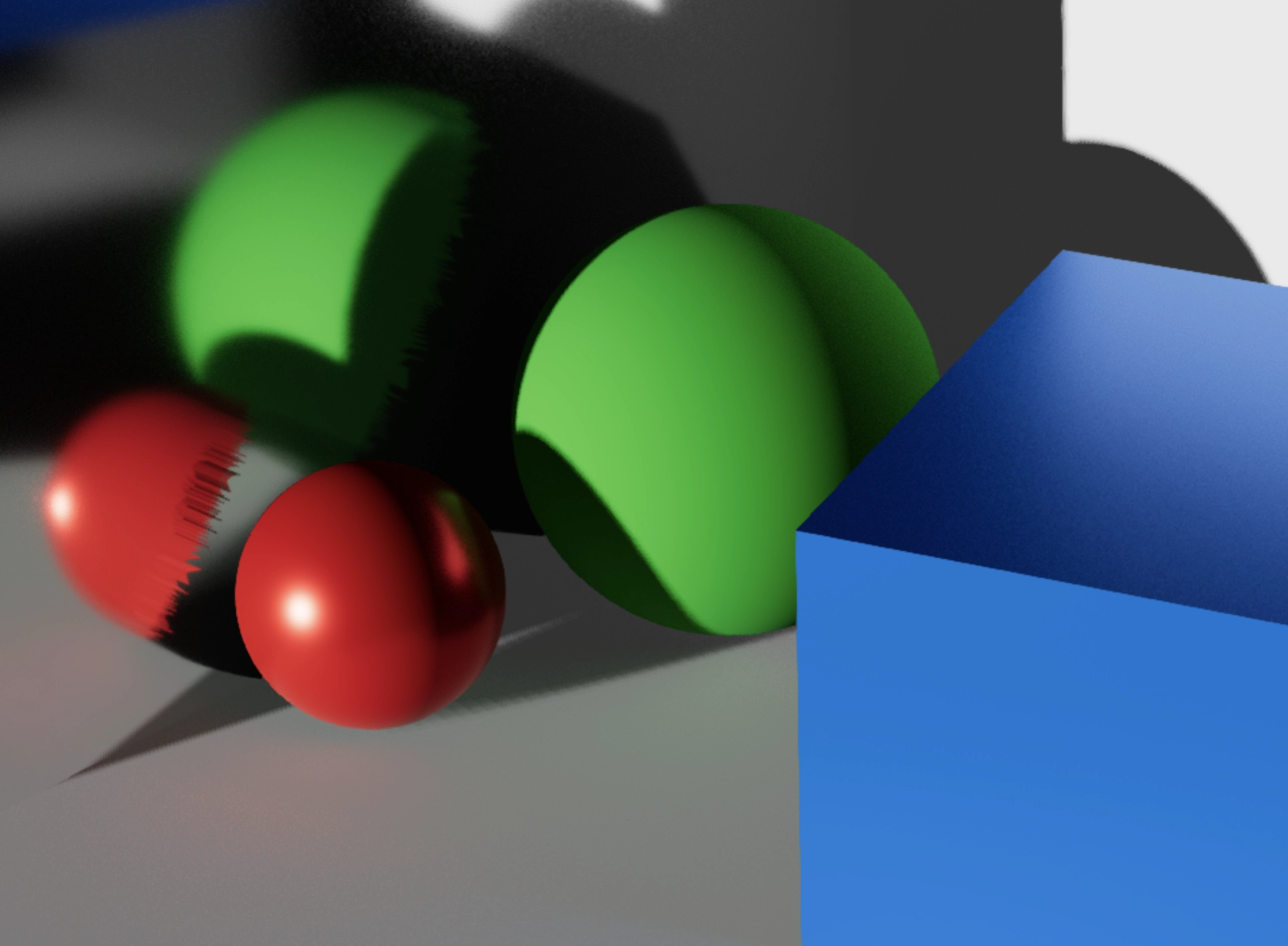
(Small parenthesis here while I'm writing this, but I really love how good the lighting and the blur of the reflection are in that picture)
At this point, I more or less cut my losses and decided to investigate an alternative approach: Probe-Based Global Illumination
When I read about this approach to Global Illumination, I knew it would solve several of my problems from the previous one.
- For one, this technique samples light using the scene’s geometry, i.e., beyond the rendered frame, by placing probes across space and tracing rays against the scene's geometry to gather light.
- It also shares lighting estimates across nearby surfaces from the probes, rather than gathering an individual estimate for every pixel in the rendered frame.
At a high level, it works as follows:
- We place probes throughout the scene. These probes act as sampling locations in world space. We will estimate indirect lighting at these positions.
- We trace rays from each probe to find intersections with the scene’s geometry.
- We compute the light arriving from those surfaces, gathering the light they reflect but also potential light they emit.
- We average the rays' contributions for each probe and store the lighting estimates.
- We read and blend the stored lighting estimate in our post-processing effect to shade visible surfaces. Occluded probes are also discarded.
- As in the previous method, we blend the indirect light with the scene’s original lighting.
The interactive diagram below illustrates each step of the probe-based approach and should give you a good mental model for what to expect in this part.
World space probes
A probe is a position we define in space where we measure something, and in our case, that something is lighting. These do not need to be defined as proper geometries, although, for learning's sake and to remain as visual as possible, we will provide an option to show them on screen.
These probes have to be defined within a set space, with boundaries (we can’t sample too loosely), which we usually set to the size of our scene where we want to observe our Global Illumination effect at play:
PROBE_MINandPROBE_MAXdefine the bounds- grid defines how many probes we will place along the
x,y, andzaxes. probeSpacingdefines how tightly those probes are packed together.
To place these probes and, as a follow-up, sample the light, we will use compute shaders. Before that compute stage, we will need to set up a few things:
- Define the storage for our probe estimates. We’ll use a 2D storage texture called an atlas where each probe stores six lighting estimates. Each estimate gathers light over a hemisphere facing one of the positive or negative coordinate axes.
1const LOBES = 6;2const width = grid[0] * LOBES;3const height = grid[1] * grid[2];
- As we did in the first section for our accumulation setup, we’ll allocate a read and a write texture and swap between them.
1const histories = [0, 1].map(() => {2const atlas = new THREE.StorageTexture(width, height);3return atlas;4});
We can now define the work our compute shader will perform. Each compute shader invocation calculates and stores one of a probe’s six directional lighting estimates. I defined an update helper function to abstract away the texture swapping and the storage step.
1const updates = histories.map((previous, index) =>2Fn(() => {3const pixel = ivec2(instanceIndex.mod(width), instanceIndex.div(width));4textureStore(5histories[1 - index],6pixel,7updateLighting(pixel, texture(previous)),8);9})().compute(width * height, [64]),10);
updateLighting is where the core of the logic resides. For a given probe, we:
- Determine the probe’s coordinate and world-space position.
- Skip the probe if it lies inside solid geometry.
- Do the same thing we did earlier: generate cosine-weighted ray directions against which we will run a
traceWorldfunction.
- For each valid intersection, we gather the surface’s emission and the sunlight it diffuses toward the probe, checking if other objects block the sunlight
1if (hit.id >= 0 && dot(hit.normal, -direction) > 0.0) {2// Handle emissive materials3incoming += shapes[hit.id].emission;45let p = origin + hit.distance * direction;6// A surface facing the sun gets more light than one at a grazing angle.7let cosine = max(dot(hit.normal, sunDirection), 0.0);89if (cosine > 0.0 && sunIntensity > 0.0) {10// Check whether sunlight can reach the hit.11let blocked = isOccluded(p + hit.normal * 0.005, sunDirection, 1000.0);1213if (!blocked) {14// For a matte material, reflected radiance is15// albedo * incoming sunlight * cosine / PI.16// Objects with high metalness will scale down / remove diffuse contributions17incoming += shapes[hit.id].albedo * (1.0 - shapes[hit.id].metalness) * (sunIntensity * cosine / 3.14159265359);18}19}20}
- Finally, we average the ray contributions. We divide the incoming light by the total number of rays, including the misses
1let fresh = incoming / f32(rays);
Then, as we did in the first part, we want to use temporal accumulation to avoid noisy estimates. We thus combine the newly computed indirect light with the previous estimates stored in the probe atlas.
1if (frame == 0u) { return vec4f(fresh, 1.0); }23let history = textureLoad(previous, pixel, 0);4let count = min(history.a + 1.0, ${HISTORY_CAP.toFixed(1)});56return vec4f(mix(history.rgb, fresh, 1.0 / count), count);
With this in place, all that’s left is to run our compute shader by dispatching the work to the GPU. You'll have the full code and implementation available in the upcoming playground. I'm purposefully skimming through some of the implementation details and parts of the wiring as they are not essential to this article.
At the end of this compute stage, we should have our probe atlas completely filled with the estimate of indirect lighting across the defined grid volume. The resulting data can be passed to the post-processing shader, which will sample and blend the estimates to render the indirect lighting reaching visible surfaces.
Rendering light from our probe atlas
As we did in the first part, we will reconstruct each visible surface’s world-space position to then find nearby probes and get the corresponding lighting estimate from the atlas
The code snippet below shows how we’re going from worldPosition for a given point to find the nearest probe and explore its neighbors in a 3 x 3 x 3 neighborhood around it:
Sampling the probe atlas
1fn sampleProbes(2atlas: texture_2d<f32>, worldPosition: vec3f,3worldNormal: vec3f, depth: f32, albedo: vec3f, enabled: f324) -> vec3f {5if (depth >= 1.0) { return vec3f(0.0); }67let n = normalize(worldNormal);89let p = worldPosition + n * 0.005;1011// Convert scene units to grid units: e.g. X = 3.25 sits between probes 3/4.12// Clamp to our finite volume; there are no extra probes beyond its bounds.13let coordinate = clamp((p - probeMin) / probeSpacing, vec3f(0.0), vec3f(gridSize - vec3i(1)));1415let base = vec3i(floor(coordinate + 0.5)) - vec3i(1);16var incoming = vec3f(0.0);17var totalWeight = 0.0;1819for (var z = 0; z < 3; z++) {20for (var y = 0; y < 3; y++) {21for (var x = 0; x < 3; x++) {22let offset = vec3i(x, y, z);23let cell = base + offset;2425if (any(cell < vec3i(0)) || any(cell >= gridSize)) { continue; }26if (textureLoad(atlas, atlasPixel(cell, 0), 0).a < 0.5) { continue; }2728let delta = probePosition(cell) - p;29let distance = length(delta);3031// Ignore probe lighting from probes on the other side of an object.32if (distance > 0.001) {33let obstruction = traceWorld(p, delta / distance);34if (obstruction.distance < distance - 0.01) { continue; }35}3637let d = abs(vec3f(cell) - coordinate);38let weights = select(390.5 * (vec3f(1.5) - d) * (vec3f(1.5) - d),40vec3f(0.75) - d * d, d < vec3f(0.5)41);42let weight = weights.x * weights.y * weights.z;43var diffuse = vec3f(0.0);4445for (var axis = 0; axis < 3; axis++) {46let lobe = axis * 2 + select(0, 1, n[axis] < 0.0);47diffuse += textureLoad(atlas, atlasPixel(cell, lobe), 0).rgb * n[axis] * n[axis];48}4950incoming += diffuse * weight;51totalWeight += weight;52}53}54}5556return albedo * incoming / max(totalWeight, 0.00001);57}
This function then acts as our lookup into the probe atlas to return the overall indirect lighting contribution for each pixel of our rendered frame. Finally, much like in the first part, all we need to do now is to add this contribution to the scene's existing lighting.
The playground below implements this first pass at our probe-based Global Illumination. You’ll find in it the complete code putting together our probe compute stage with our final effect:
Notice how:
- We do still have colored surfaces contributing light to surrounding surfaces
- We get a decent output at a lower performance cost. Even with a loose probe grid and fewer rays, the effect is noticeable and adds a lot to the scene’s beautiful lighting and realism.
- Moving the camera preserves the probe’s lighting and history! This is a big win compared to the screen-space Global Illumination counterpart we saw earlier
- The lighting is, however, a bit less accurate. Maybe this scene is not the best to surface that, but the indirect light is just softer and less precise.
- We can now have off-screen light, or emitters, and those will be taken into account from the get-go.
- A denser grid can capture smaller changes in lighting, but costs more in probe updatyes and storage.
Despite its flaws, it ended up being more usable for my projects. Oh also, you should try to toggle the night mode to see how emissive surfaces also contribute to the scene's indirect lighting, which we got almost for free with the current implementation. No additional tracing necessary!
1// 0 if day, 1 if night2incoming += shapes[hit.id].emission * nightTime;
However, you'll quickly notice that, if we move the light in the scene above, the entire lighting history is thrown away, and our compute stage has to start accumulating light from zero again. We need to solve for this.
Hysteresis
One solution to the issue we’re facing here is simply to not discard our previous estimates when our light moves. Of course, there’s a twist, because keeping it all would end up preserving outdated lighting, so we need to decide how much history to retain:
- Too little of it, and we would end up with noise once again
- Too much, and the updates would be slow to respond
Hysteresis controls how much of our previous indirect lighting estimate we blend into the new one. A higher value reduces noise but makes our indirect lighting adapt more slowly when the light moves. The widget below demonstrates its effect:
The main change that benefits us happens at the end of our compute shader.
Updated updateLighting function with hysteresis
1if (frame == 0u) { return vec4f(fresh, 1.0); }23let history = textureLoad(previous, pixel, 0);4-let count = min(history.a + 1.0, ${HISTORY_CAP.toFixed(1)});5+let count = min(history.a + 1.0, ${PERSISTENT_HISTORY_CAP.toFixed(1)});67-return vec4f(mix(history.rgb, fresh, 1.0 / count), count);8+let window = min(9+ 1.0 / (1.0 - hysteresis) + f32(stableFrames),10+ ${PERSISTENT_HISTORY_CAP.toFixed(1)}11+);12+let retention = min(1.0 - 1.0 / window, 1.0 - 1.0 / count);13+14+return vec4f(mix(fresh, history.rgb, retention), count);
Here, we still read previous estimates from the probe atlas, but instead of determining its influence only from the accumulated count, we also calculate a new retention weight for our history.
- With hysteresis set to 0.95, once enough history has accumulated, the blend consists of 95% history and 5% updated measurements. While the lighting remains unchanged, we give history progressively more influence.
- While lighting remains unchanged,
stableFramesincreases, giving history more weight. - When lighting changes,
stableFramesis reset without clearing the atlas, allowing probes to make new measurements that gradually replace the old lighting instead of starting from scratch.
Below is an updated version of our scene featuring probe-based Global Illumination, this time, with hysteresis.
Probe-based Global Illumination does give us a decent result overall. We fixed many of the caveats of SSGI that were bothering me. Yes, there still is some ghosting when the light changes abruptly, but for my use case, which centers around almost static/slowly changing lights, it does what I need it to do. The only "downside" is that I grew quite fond of the noise produced by the raymarching, which here is absent. If like me, you miss it a bit too much, you can always re-introduce it through an additional grain post-processing pass.
The work we’ve done in the previous part provides indirect lighting that gradually updates when the lighting changes, and remains stable while the camera moves, all that with a noise-less output that performs pretty well.
There are still a few things we can add to bring this effect together:
- We’ll start with reflections. With world-space tracing already in place, we can now find surfaces hidden from the camera and reuse our probes to light their reflections, something that, like we saw in an example earlier, would have only yielded black pixels in screen space.
- Then, we should let the sky contribute to our indirect lighting. Using atmospheric scattering, this would bring a natural tint to the scene and let us have dynamic lighting as the sun moves across the sky, including sunset/sunrise colors.
Tracing reflections
Adding support for reflections consists of a few steps:
- We need to trace a reflected ray.
- Find the surface it hits.
- Compute its direct and indirect lighting.
We start from a visible surface point; we reflect the viewing direction around its normal and trace a ray into the scene. The surface we hit from this process gives us the light we’ll see reflected in that point.
Once we’ve found that surface, we can compute its lighting by combining emissions, direct lighting, and indirect lighting by sampling our probe atlas as we did in the previous part.
However, before all that, we need to take into account the properties of the materials receiving reflections. The code snippet below adds an extra render target to store the roughness and metalness of each material present in the
Add render target to track material properties
1const scenePass = pass(scene, camera, { samples: 0 });2scenePass.setMRT(3mrt({4output,5normal: normalWorld,6albedo: mix(diffuseColor, materialColor, materialMetalness),7material: vec4(roughness, materialMetalness, 0, 1),8}),9)
Reflections can be handled through a dedicated traceReflection function that we can then add to our post-processing shader
Trace the reflection from a given camera world position
1fn traceReflection(2atlas: texture_2d<f32>, sky: texture_2d<f32>, worldPosition: vec3f, worldNormal: vec3f,3cameraPosition: vec3f, depth: f32, albedo: vec3f, material: vec2f,4sunDirection: vec3f, sunRadiance: vec3f, nightTime: f32,5) -> vec3f {6if (depth >= 1.0 || enabled < 0.5) { return vec3f(0.0); }78let roughness = clamp(material.x, 0.0, 1.0);9let metalness = clamp(material.y, 0.0, 1.0);1011// First teaching step: sharp reflections only. This fades the mirror term12// on rough materials; it is NOT GGX roughness blur or a full rough BRDF.13let mirrorWeight = (1.0 - roughness) * (1.0 - roughness);1415// Skip surfaces whose sharp reflection contribution is negligible.16if (mirrorWeight < 0.0001) { return vec3f(0.0); }1718let n = normalize(worldNormal);19let v = normalize(cameraPosition - worldPosition);20// Schlick Fresnel: metals tint reflections; grazing angles reflect more.21let f0 = mix(vec3f(0.04), albedo, metalness);22let fresnel = f0 + (vec3f(1.0) - f0) * pow(1.0 - clamp(dot(n, v), 0.0, 1.0), 5.0);2324// Tracing reflection rays25let origin = worldPosition + n * 0.005;26let direction = reflect(-v, n);27let hit = traceWorld(origin, direction);2829// A reflected view that misses geometry sees the same directional background as30// the camera. This is a visual fallback, not environment lighting for probes.31if (hit.id < 0) {32// returning null here, but we will return the background sky or scene in the next part33return vec3(0.0);34}35if (dot(hit.normal, -direction) <= 0.0) { return vec3f(0.0); }3637// World-space position of the surface hit by the reflection38let p = origin + direction * hit.distance;39let surface = shapes[hit.id];40let diffuseAlbedo = surface.albedo * (1.0 - surface.metalness);41var radiance = surface.emission * nightTime;42let cosine = max(dot(hit.normal, sunDirection), 0.0);43if (cosine > 0.0 && any(sunRadiance > vec3f(0.0))) {44let blocked = isOccluded(p + hit.normal * 0.005, sunDirection, 1000.0);45if (!blocked) {46radiance += diffuseAlbedo * (sunRadiance * cosine / 3.14159265359);47}48}4950// Sample indirect light51radiance += sampleProbes(atlas, p, hit.normal, 0.0, diffuseAlbedo);5253// Only one reflection hit: reflected surfaces contribute emission and54// diffuse lighting, not another mirror ray (no recursive reflections yet).55return radiance * fresnel * mirrorWeight;56}
The returned value represents the reflection’s final light contribution at the original surface point worldPosition:
radianceis the light coming from the surface the reflected ray hits, such as its emissive light and its direct/indirect light.fresnelrepresents how much of that light we reflect based on the viewing angle.mirrorWeightis the factor for the strength of the reflection based on roughness.
The only thing remaining is to do is to add it to the final combined light:
1const combined = vec4(2sceneColor.add(indirect).add(reflection),31,4);
I made the small playground below to quickly demonstrate this new addition to our Global Illumination post-processing effect:
Adding sky light
During my learning journey, I could not stop thinking about ways I could include some of my earlier work around lighting, and my atmospheric scattering shader work to have that beautiful blue sky in my scene. However, it was deceptively complex: I had to have the sky as a backdrop and also have its color / light contribute to the scene as the sun moves and thus be taken into account when we're gathering indirect lighting.
I was tempted to include the atmospheric scattering math into my probe ray logic, but instead, I decided to put it in its own compute shader, to only run it when necessary, as in my use case, the sky won't change that much (unless I change the position of the sun, but that's an acceptable dependency).
For each pixel in the texture, we take a direction it points to in the sky, then call atmosphere (abstracted atmospheric scattering logic) to calculate the color and intensity of the light coming from that direction.
Compute the color of the sky and its light at a given direction
1fn skyTexel(pixel: vec2i, sunDirection: vec3f, intensity: f32, haze: f32) -> vec4f {2let uv = (vec2f(pixel) + 0.5) / vec2f(${SKY_WIDTH.toFixed(1)}, ${SKY_HEIGHT.toFixed(1)});3let phi = (uv.x - 0.5) * 2.0 * skyPI;4let theta = uv.y * skyPI;5let direction = vec3f(sin(theta) * cos(phi), cos(theta), sin(theta) * sin(phi));67return vec4f(atmosphere(direction, sunDirection, intensity, haze), 1.0);8}
After that, we can sample the resulting sky texture when tracing probes:
Sampling the sky color and light intensity
1fn sampleSky(sky: texture_2d<f32>, direction: vec3f) -> vec3f {2let d = normalize(direction);3// Cosine samples can land exactly on a pole. atan2(0, 0) is undefined4// on the GPU and would contaminate every later temporal average.5var longitude = 0.0;6if (abs(d.x) + abs(d.z) > 0.000001) {7longitude = atan2(d.z, d.x);8}9let uv = vec2f(longitude / 6.28318530718 + 0.5, acos(clamp(d.y, -1.0, 1.0)) / 3.14159265359);10let pixel = uv * vec2f(textureDimensions(sky)) - 0.5;11let base = vec2i(floor(pixel));12let blend = fract(pixel);1314return mix(15mix(skyLoad(sky, base), skyLoad(sky, base + vec2i(1, 0)), blend.x),16mix(skyLoad(sky, base + vec2i(0, 1)), skyLoad(sky, base + vec2i(1, 1)), blend.x),17blend.y18);19}
Finally, this function can be called within probeUpdate shader whenever a ray misses a surface / scene geometry. It will add the light arriving from that direction to the probe’s lighting estimate, instead of keeping the contribution at 0.0.
Including sky light to our probe atlas
1if (hit.id >= 0 && dot(hit.normal, -direction) > 0.0) {2// Handle standard surface hits3}4+5+if (hit.id < 0) {6+ incoming += sampleSky(sky, direction);7+}
We should also not forget to update our reflection logic from the previous section. Previously, when a reflected ray missed a surface, we’d return a constant color as a pixel, or simply vec3(0.0), i.e., black. Now we can sample the sky in that direction:
Sampling the sky when reflections don't hit a surface
1if (hit.id < 0) {2- // returning null here, but we will return the background sky or scene in the next part3- return vec3(0.0);4+ return sampleSky(sky, direction) * fresnel * mirrorWeight;5}
Including this, alongside some extra wiring and details that are not very interesting, in our demo from earlier gives us:
- a beautiful sky blue backdrop (which I can't get enough of)
- a very accurate and natural-looking sky light contribution to the scene
- naturally tinted shadows, more soft, less "in your face"
I added arch geometries in this demo as I did for my own scene from mid-October 2026.

had this idea of combining my atmosphere shader work with global illumination also got reflections working the sky contributes beautifully to the overall lighting of this scene as the sun moves, all in real time in the browser https://t.co/ohJgRRC1Pz https://t.co/Vk0rSRRtlm
I included the proper intersection logic in the traceWorld function in the demo above, it's a bit gnarly though. In the future, I’d like, and recommend, tracing against triangle meshes via a BVH, as mentioned earlier, making it easier to handle more complex geometries.
Final Thoughts
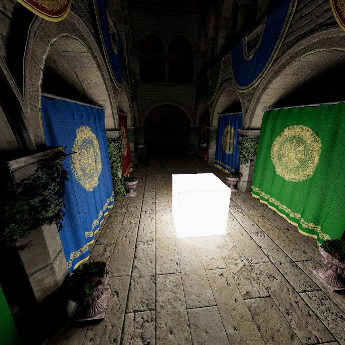
I’m still solving for some of the pitfalls of this implementation as of writting this; it’s definitely not production-grade in any way (check out the probe-based GI included in Three.js for a more usable implementation!), but I'm nonetheless very happy with the result especially given how interesting it was to get a better grasp of what’s happening behind the scenes with those more advanced lighting techniques. If you want to follow what the pros are working on at the edge, you should also check out the work of @CodyBennett on Radiance Cascade, another GI technique I still haven't looked much into (it's on my list). I’m always very excited to see his progress:

Noiseless glossy specular global illumination (single bounce) with Radiance Cascades by directly observing the cascade data with a split-sum approximation. No additional rays are traced here, and light transport remains independent of scene complexity and material properties. https://t.co/q7U2JCyia0
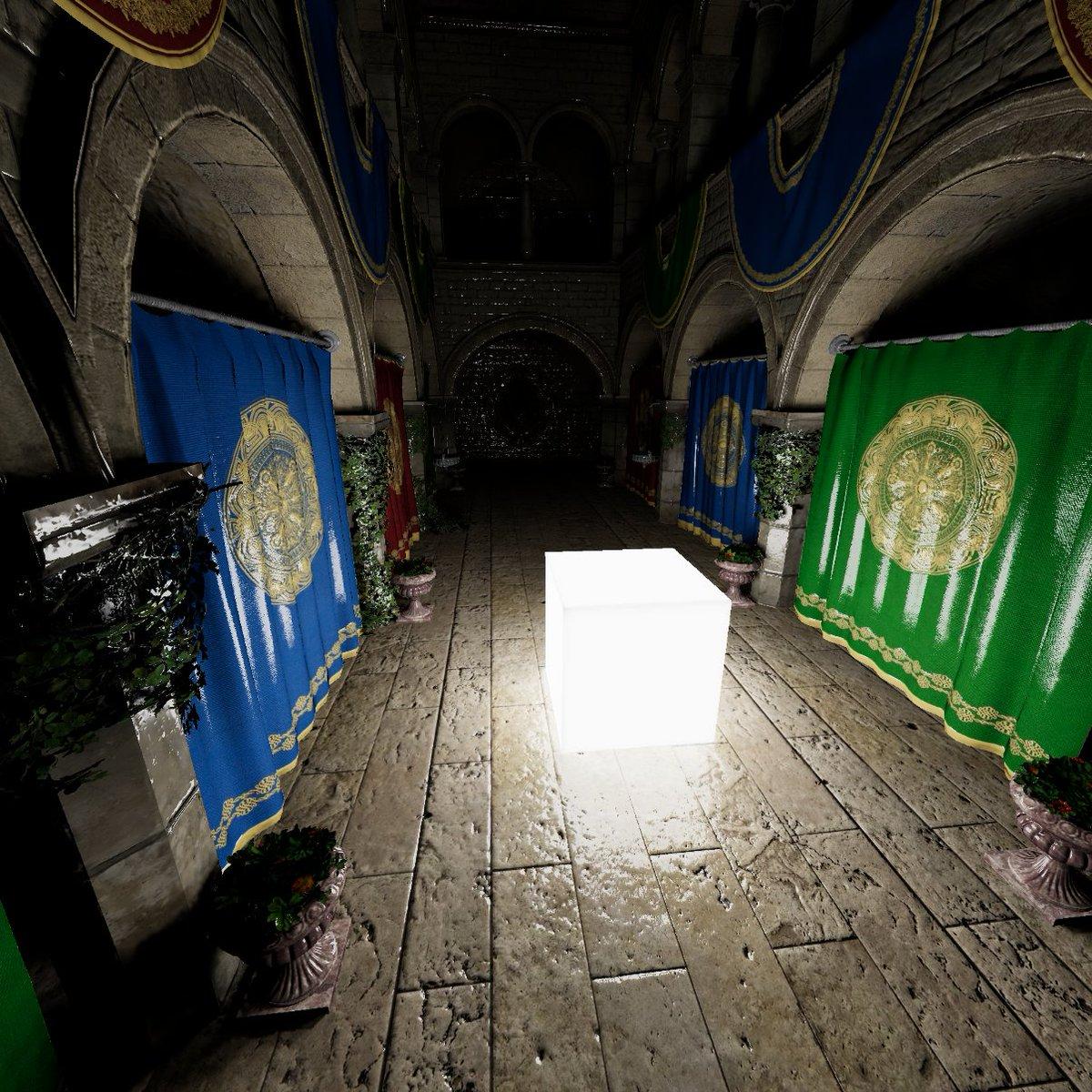
Teaching myself the basics of Global Illumination was a great way to appreciate the outsized impact indirect lighting. I’m also very much looking forward to using it on my upcoming projects and mix-and-match it with some of my past work that, despite putting a lot of work into it, was always a bit disappointing in the end. The cool thing with lighting effects overall is that they can stack quite well, so some of the obvious next step is to combine GI with things like caustics, glass effects, or even Volumetric Lighting like I did earlier this fall:
a sneak peek at my recent global illumination work color bleeding, light bounces... love spending an obscene amount of time on these effects :), they are so satisfying to get right https://t.co/aDctq7cufF https://t.co/fUD9xu8wBn
I’ll now get back to building and trying new things around shaders, lighting, effects, and materials, and hope that while waiting for the next write-up, this walkthrough on Global Illumination will be helpful to you and give you a renewed appreciation for the tiny details that make all the difference.
Path tracing is a rendering algorithm in computer graphics that simulates how light interacts with objects and participating media to generate realistic [...] images. Source.
One of my earliest use cases of the Blinn-Phong lighting model was for Refraction, dispersion, and other shader light effects.
Color bleeding is a lighting phenomenon where strong saturated colored objects tend to have their colors reflected off a surface. It adds a "tint" to neighboring surfaces.
I highly recommend reading these in order if you're curious about some of the implementationn details that I'm overlooking here, see On Rendering the Sky, Sunsets, and Planets and On Shaping Light: Real-Time Volumetric Lighting with Post-Processing and Raymarching for the Web.
See Coordinate systems and transformations for a detailed breakdown of the process.
I first talked about the method in The Magical World of Particles with React Three Fiber and Shaders.