Real-time dreamy Cloudscapes with Volumetric Raymarching
I spent the past few months diving into the realm of Raymarching and studying some of its applications that may come in handy for future 3D projects, and while I managed to build a pretty diverse set of scenes, all of them consisted of rendering surfaces or solid objects. My blog post on Raymarching covered some of the many impressive capabilities of this rendering technique, and as I mentioned at the end of that post, that was only the tip of the iceberg; there is a lot more we can do with it.
One fascinating aspect of Raymarching I quickly encountered in my study was its capacity to be tweaked to render volumes. Instead of stopping the raymarched loop once the ray hits a surface, we push through and continue the process to sample the inside of an object. That is where my obsession with volumetric clouds started, and I think the countless hours I spent exploring the many Sky Islands in Zelda Tears of the Kingdom contributed a lot to my curiosity to learn more about how they work. I thus studied a lot of Shadertoy scenes such as "Clouds" by Inigo Quilez, "Starry Night" by al-ro, and "Volumetric Raymarching sample" by Suyoku leveraging many Volumetric Raymarching techniques to render smoke, clouds, and cloudscapes, which I obviously couldn't resist giving a try rebuilding myself:
I spent a great deal of time exploring the different ways I could use Raymarching to render clouds, from fully wrapping my head around the basics of Volumetric Raymarching to leveraging physically based properties of clouds to try getting a more realistic output while also trying to squeeze as much performance out of my scenes with neat performance improvement tips I learned along the way. I cover all of that in this article, which I hope can serve you as a field guide for your own volumetric rendering experiments and learnings.
In my previous blog post on Raymarching, we saw that the technique relied on:
- Signed Distance Fields: functions that return the distance of a given point in space to the surface of an object
- A Raymarching loop where we march step-by-step alongside rays cast from an origin point (a camera, the observer's eye) through each pixel of an output image, and we calculate the distance to the object's surface using our SDF. Once that distance is small enough, we can draw a pixel.
If you've practiced this technique on some of your own scenes, you're in luck: Volumetric Raymarching relies on the same principles: there's a loop, rays cast from an origin, and SDFs. However, since we're rendering volumes instead of surfaces, there's a tiny twist to the technique 👀.
How to sample a volume
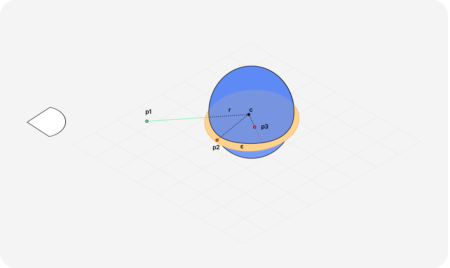
The first time we got introduced to the concept of SDF, we learned that it was important not to step inside the object during our Raymarching loop to have a beautiful render. I even emphasized that fact in one of my diagrams showcasing 3 points relative to an object:
P1is located far from the surface, in green, representing a positive distance to the surface.P2is located at a close distance ε to the surface, in orange,P3positioned inside the object, in red, representing a negative distance to the surface.
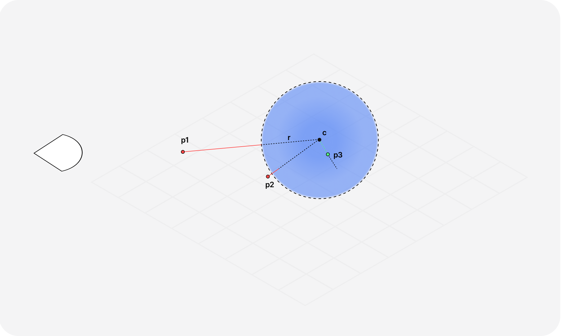
When sampling a volume, we'll need to actually raymarch inside our object and reframe how we think of SDF: instead of representing the distance to the surface, we will now use it as the density of our volume.
- When raymarching outside, the density is null, or
0. - Once we raymarch inside, it is positive.
To illustrate this new way of thinking about Raymarching in the context of volume, here's a modified version of the widget I introduced in my blog post on the topic earlier this year.
That reframing of what an SDF represents ends up changing two core principles in our Raymarching technique that will have to be reflected in our code:
- We have to march step-by-step with a constant step size along our rays. We no longer use the distance returned by the SDF.
- Our SDF now returns the opposite of the distance to the surface to properly represent the density of our object (positive on the inside,
0on the outside)
Our first Volumetric Raymarching scene
Now that we have a grasp of sampling volumes using what we know about Raymarching, we can try implementing it by modifying an existing scene. For brevity, I'm not detailing the setup of a basic of Raymarching scenes. If you want a good starting point you can head to my Raymarching setup I already introduced in a previous article.
The setup of the scene is quite similar to what we're familiar with in classic Raymarching; the modifications we'll need to do are located in:
- Our SDF functions: we'll need to return the opposite of the distance:
-dinstead ofd.
Example of SDF used in Volumetric Raymarching
1float sdSphere(vec3 p, float radius) {2return length(p) - radius;3}45float scene(vec3 p) {6float distance = sdSphere(p, 1.0);7return -distance;8}
- Our
raymarchfunction: we'll need to march at a constant step size and start drawing only once the density is over 0.
Volumetric Raymarching loop with constant step size
1#define MAX_STEPS 10023const float MARCH_SIZE = 0.08;4//...56float depth = 0.0;7vec3 p = rayOrigin + depth * rayDirection;89vec4 res = vec4(0.0);1011for (int i = 0; i < MAX_STEPS; i++) {12float density = scene(p);13if (density > 0.0) {14// ...15}1617depth += MARCH_SIZE;18p = rayOrigin + depth * rayDirection;19}
Now comes another question: what shall we draw once our density is positive to represent a volume?
For this first example, we can keep things simple and play with the alpha channel of our colors to make it proportional to the density of our volume: the denser our object gets as we march into it, the more opaque/darker it will be.
Simple Volumetric Raymarching loop
1const float MARCH_SIZE = 0.08;23vec4 raymarch(vec3 rayOrigin, vec3 rayDirection) {4float depth = 0.0;5vec3 p = rayOrigin + depth * rayDirection;67vec4 res = vec4(0.0);89for (int i = 0; i < MAX_STEPS; i++) {10float density = scene(p);1112// We only draw the density if it's greater than 013if (density > 0.0) {14vec4 color = vec4(mix(vec3(1.0,1.0,1.0), vec3(0.0, 0.0, 0.0), density), density );15color.rgb *= color.a;16res += color * (1.0 - res.a);17}1819depth += MARCH_SIZE;20p = rayOrigin + depth * rayDirection;21}2223return res;24}
If we try to render this code in our React Three Fiber canvas, we should get the following result 👀
We now know and applied the basics of Volumetric Raymarching. So far, we only rendered a simple volumetric sphere with constant density as we march through the volume, which is a good start. We can now try using that simple scene as a foundation to render something more interesting: clouds!
Noisy Volume
Going from our simple SDF of a sphere to a cloud consists of drawing it with a bit more noise. Clouds don't have a uniform shape nor do they have a uniform density, thus we need to introduce some organic randomness through noise in our Raymarching loop. If you read some of my previous articles, you should already be familiar with the concept of:
- Noise, Perlin noise, and value noise derivative
- Fractal Brownian Motion, or FBM.
- Texture based noise.
To generate raymarched landscapes, we used a noise texture, noise derivatives, and FBM to get a detailed organic result. We'll rely on some of those concepts to create organic randomness and obtain a cloud from our SDF ☁️.
Noise function for Raymarched landscape
1vec3 noise(vec2 x) {2vec2 p = floor(x);3vec2 f = fract(x);4vec2 u = f * f * (3. - 2. * f);56float a = textureLod(uTexture, (p + vec2(.0,.0)) / 256.,0.).x;7float b = textureLod(uTexture, (p + vec2(1.0,.0)) / 256.,0.).x;8float c = textureLod(uTexture, (p + vec2(.0,1.0)) / 256.,0.).x;9float d = textureLod(uTexture, (p + vec2(1.0,1.0)) / 256.,0.).x;1011float noiseValue = a + (b-a) * u.x + (c-a) * u.y + (a - b - c + d) * u.x * u.y;12vec2 noiseDerivative = 6. * f * (1. - f) * (vec2(b - a, c - a) + (a - b - c + d) * u.yx);1314return vec3(noiseValue, noiseDerivative);15}
For clouds, our noise function looks a bit different:
Noise function for Volumetric clouds
1float noise(vec3 x ) {2vec3 p = floor(x);3vec3 f = fract(x);4vec2 u = f * f * (3. - 2. * f);56vec2 uv = (p.xy + vec2(37.0, 239.0) * p.z) + u.xy;7vec2 tex = textureLod(uNoise,(uv + 0.5) / 256.0, 0.0).yx;89return mix( tex.x, tex.y, u.z ) * 2.0 - 1.0;10}
To tell you the truth, I saw this function in many Shadertoy demos without necessarily seeing a credited author or even a link to an explanation; I kept using it throughout my work as it still yielded a convincing cloud noise pattern. Here's an attempt at gathering together some of its specificities from my own understanding:
- Clouds are 3D structures, so our function takes in a
vec3as input: a point in space within our cloud. - The texture lookup differs from its landscape counterpart: we're sampling it as a 2D slice from a 3D position. The
vec2(37.0, 239.0) * p.zseems a bit arbitrary to me, but from what I gathered, it allows for more variation in the resulting noise. - We then mix two noise values from our texture lookup based on the
zvalue to generate a smooth noise pattern and rescale it within the[-1, 1]range.
Applying this noise along with a Fractal Brownian motion is pretty similar to what we're used to with Raymarched landscapes:
Fractal Brownian Motion applied to our Volumetric Raymarching scene
1float fbm(vec3 p) {2vec3 q = p + uTime * 0.5 * vec3(1.0, -0.2, -1.0);3float g = noise(q);45float f = 0.0;6float scale = 0.5;7float factor = 2.02;89for (int i = 0; i < 6; i++) {10f += scale * noise(q);11q *= factor;12factor += 0.21;13scale *= 0.5;14}1516return f;17}1819float scene(vec3 p) {20float distance = sdSphere(p, 1.0);21float f = fbm(p);2223return -distance + f;24}
If we apply the code above to our previous demo, we do get something that starts to look like a cloud 👀:
Adding light
Once again, we're just "starting" to see something approaching our goal, but a crucial element is missing to make our cloud feel more cloudy: light.
The demo we just saw in the previous part lacks depth and shadows and thus doesn't feel very realistic overall, and that's due to the lack of diffuse light.
To add light to our cloud and consequentially obtain better shadows, one may want to apply the same lighting we used in standard Raymarching scenes:
- Calculate the normal of each sample point using our
scenefunction - Use the dot product of the normal and the light direction
Diffuse lighting in Raymarched scene using normals
1vec3 getNormal(vec3 p) {2vec2 e = vec2(.01, 0);34vec3 n = scene(p) - vec3(5scene(p-e.xyy),6scene(p-e.yxy),7scene(p-e.yyx));89return normalize(n);10}1112void main() {13// ...1415vec3 ro = vec3(0.0, 0.0, 5.0);16vec3 rd = normalize(vec3(uv, -1.0));17vec3 lightPosition = vec3(1.0);1819float d = raymarch(ro, rd);20vec3 p = ro + rd * d;212223vec3 color = vec3(0.0);2425if(d<MAX_DIST) {26vec3 normal = getNormal(p);27vec3 lightDirection = normalize(lightPosition - p);2829float diffuse = max(dot(normal, lightDirection), 0.0);30color = vec3(1.0, 1.0, 1.0) * diffuse;31}3233gl_FragColor = vec4(color, 1.0);34}
That would work in theory, but it's not the optimal choice for Volumetric Raymarching:
- The
getNormalfunction requires a lot of sample points to estimate the "gradient" in every direction. In the code above, we need 4, but there are code snippets that require 6 for a more accurate result. - Our volumetric raymarching loop is more resource-intensive: we're walking at a constant step size along our ray to sample the density of our volume.
Thus, we need another method or approximation for our diffuse light. Luckily, Inigo Quilez presents a technique to solve this problem in his article on directional derivatives. Instead of having to sample our density in every direction like getNormal, this method simplifies the problem by sampling the density at our sampling point p and at an offset in the direction of the light and getting the difference between those values to approximate how the light scatters roughly inside our volume.
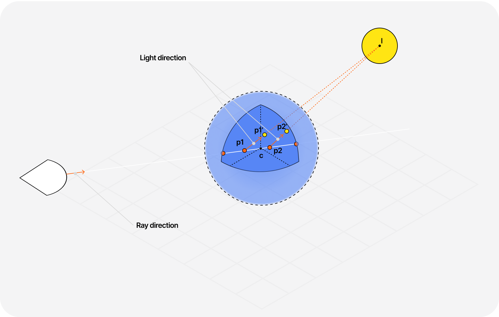
In the diagram above, you can see that we're sampling our density at p1 and at another point p1' that's a bit further along the light ray:
- If the density increases along that path, that means the volume gets denser, and light will scatter more
- If the density gets smaller, our cloud is less thick, and thus, the light will scatter less.
This method only requires 2 sampling points and consequentially requires fewer resources to give us a good approximation of how the light behaves with the volume around p1.
We can apply this diffuse formula to our demo as follows:
Diffuse lighting using directional derivatives
1//...2if (density > 0.0) {3// Directional derivative4// For fast diffuse lighting5float diffuse = clamp((scene(p) - scene(p + 0.3 * sunDirection)) / 0.3, 0.0, 1.0 );67vec3 lin = vec3(0.60,0.60,0.75) * 1.1 + 0.8 * vec3(1.0,0.6,0.3) * diffuse;8vec4 color = vec4(mix(vec3(1.0, 1.0, 1.0), vec3(0.0, 0.0, 0.0), density), density );9color.rgb *= lin;1011color.rgb *= color.a;12res += color * (1.0 - res.a);13}14//...
That is, once again, very similar to what we were doing in standard Raymarching, except that now, we have to include it inside the Raymarching loop as we're sampling a volume and thus have to run the calculation multiple times throughout the volume as the density may vary whereas a surface required only one diffuse lighting computation (at the surface).
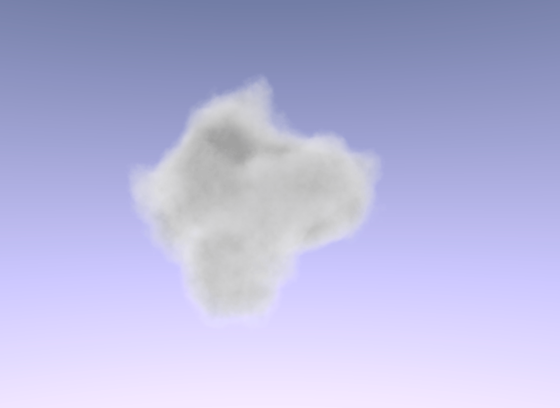
You can observe the difference between our cloud without lighting and with diffuse lighting below 👇
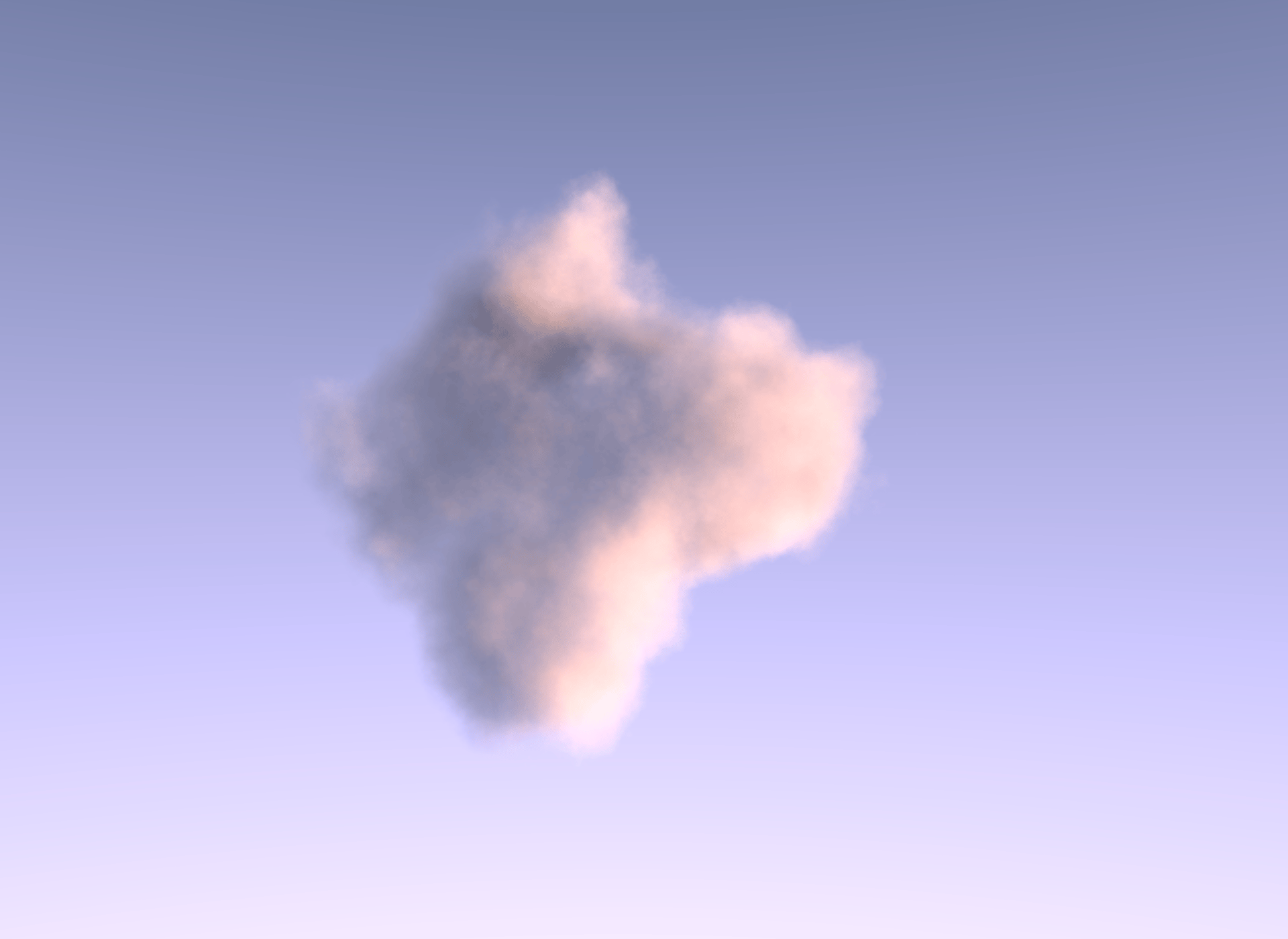
And here's the demo featuring the concept and code we just introduced 👀:
Morphing clouds
Let's take a little break to tweak our scene and have some fun with what we built so far! Despite the differences between the standard Raymarching and its volumetric counterpart, there are still a lot of SDF-related concepts you can apply when building cloudscapes.
You can try to make a cloud in fun shapes like a cross or a torus, or even better, try to make it morph from one form to another over time:
Mixing SDF to morph volumetric clouds into different shapes
1mat2 rotate2D(float a) {2float s = sin(a);3float c = cos(a);4return mat2(c, -s, s, c);5}67float nextStep(float t, float len, float smo) {8float tt = mod(t += smo, len);9float stp = floor(t / len) - 1.0;10return smoothstep(0.0, smo, tt) + stp;11}1213float scene(vec3 p) {14vec3 p1 = p;15p1.xz *= rotate2D(-PI * 0.1);16p1.yz *= rotate2D(PI * 0.3);1718float s1 = sdTorus(p1, vec2(1.3, 0.9));19float s2 = sdCross(p1 * 2.0, 0.6);20float s3 = sdSphere(p, 1.5);21float s4 = sdCapsule(p, vec3(-2.0, -1.5, 0.0), vec3(2.0, 1.5, 0.0), 1.0);2223float t = mod(nextStep(uTime, 3.0, 1.2), 4.0);2425float distance = mix(s1, s2, clamp(t, 0.0, 1.0));26distance = mix(distance, s3, clamp(t - 1.0, 0.0, 1.0));27distance = mix(distance, s4, clamp(t - 2.0, 0.0, 1.0));28distance = mix(distance, s1, clamp(t - 3.0, 0.0, 1.0));2930float f = fbm(p);3132return -distance + f;33}
This demo is a reproduction of this volumetric rendering related Shadertoy scene. I really like this creation because the result is very organic, and it gives the impression that the cloud is rolling into its next shape naturally.
You can also try to render:
- Clouds merging together using the
minandsmoothminof two SDFs - Repeating clouds through space using the
modfunction
There are a lot of creative compositions to try!
You may notice that running the scenes we built so far may make your computer sound like a jet engine at high resolution or at least not look as smooth as they could. Luckily, we can do something about it and use some performance optimization techniques to strike the right balance between FPS count and output quality.
Blue noise dithering
One of the main performance pitfalls of our current raymarched cloudscape scene is due to:
- the number of steps we have to perform to sample our volume and the small
marchSize - some heavy computation we have to do within our loop, like our directional derivative or FBM.
This issue will only worsen as we attempt to make more computations to achieve a more physically accurate output in the next part of this article.
One of the first things we could do to make this scene more efficient would be to reduce the amount of steps we perform when sampling our cloud and increase the step size. However, if we attempt this on some of our previous examples (I invite you to try), some layering will be visible, and our volume will look more like some kind of milk soup than a fluffy cloud.
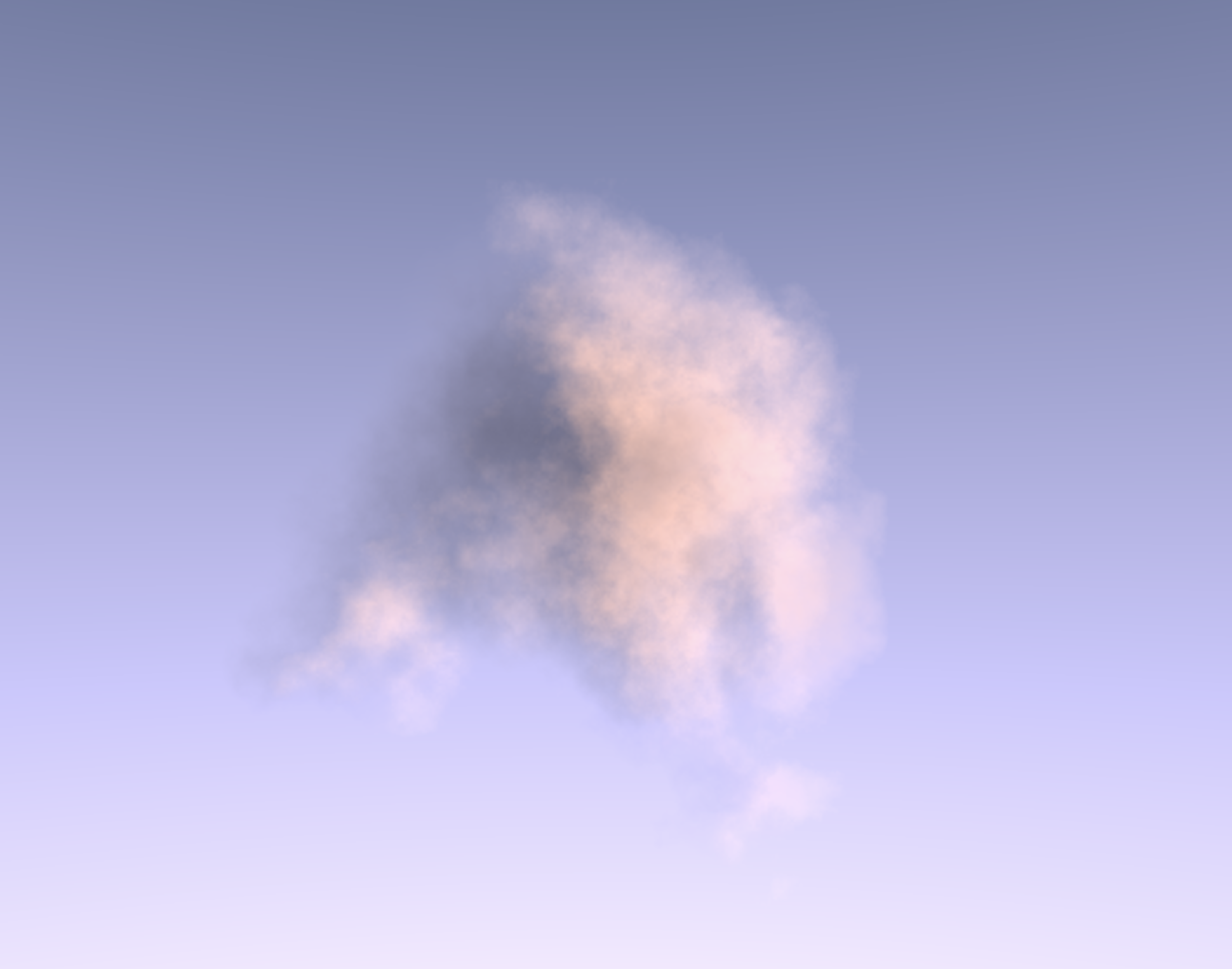
You might have encountered the concept of dithering or some images using dithering styles before. This process can create the illusion of more colors or shades in an image than available or purely used for artistic ends. I recommend reading Dithering on the GPU from Alex Charlton if you want a quick introduction.
In Ray marching fog with blue noise, the author showcases how you can leverage blue noise dithering in your raymarched scene to erase the banding or layering effect due to a lower step count or less granular loop. This technique leverages a blue noise pattern, which has fewer patterns or clumps than other noises and is less visible to the human eye, to obtain a random number each time our fragment shader runs. We then introduce that number as an offset at the beginning of the raymarched loop, moving our sampling start point along our ray for each pixel of our output.

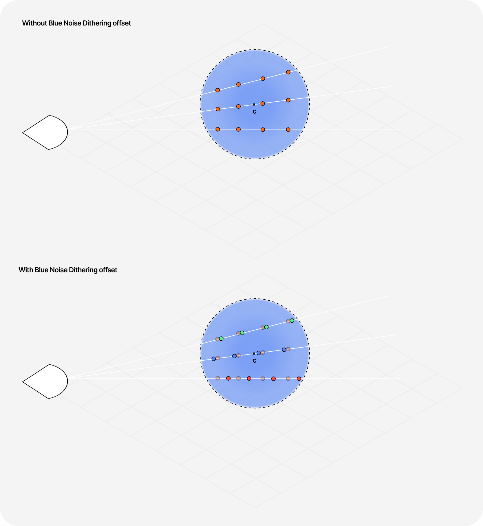
Blue noise dithering introducing an offset in our Raymarching loop
1uniform sampler2D uBlueNoise;23//...45vec4 raymarch(vec3 rayOrigin, vec3 rayDirection, float offset) {6float depth = 0.0;7depth += MARCH_SIZE * offset;8vec3 p = rayOrigin + depth * rayDirection;9//...10}1112void(main) {13//...14float blueNoise = texture2D(uBlueNoise, gl_FragCoord.xy / 1024.0).r;15float offset = fract(blueNoise);1617vec4 res = raymarch(ro, rd, offset);18//...19}
By introducing some blue noise dithering in our fragment shader, we can erase those artifacts and get a high-quality output while maintaining the Raymarching step count low!
However, under some circumstances, the dithering pattern can be pretty noticeable. By looking at some other Shadertoy examples, I discovered that introducing a temporal aspect to the blue noise can attenuate this issue.
Temporal blue noise dithering offset
1float offset = fract(blueNoise + float(uFrame%32) / sqrt(0.5));
Here's a before/after comparison of our single frame of our raymarched cloud. I guess the results speak for themselves here 😄.
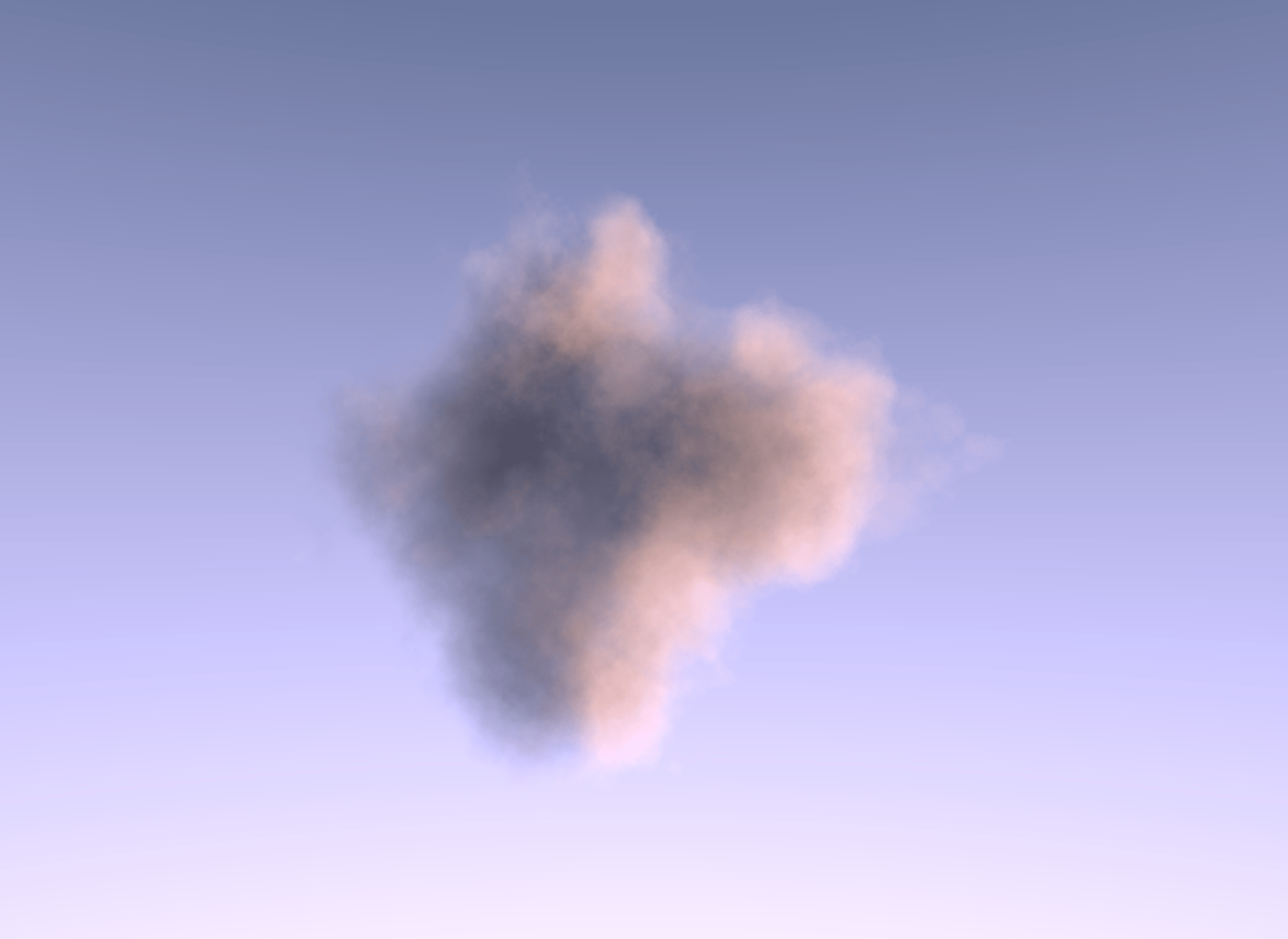
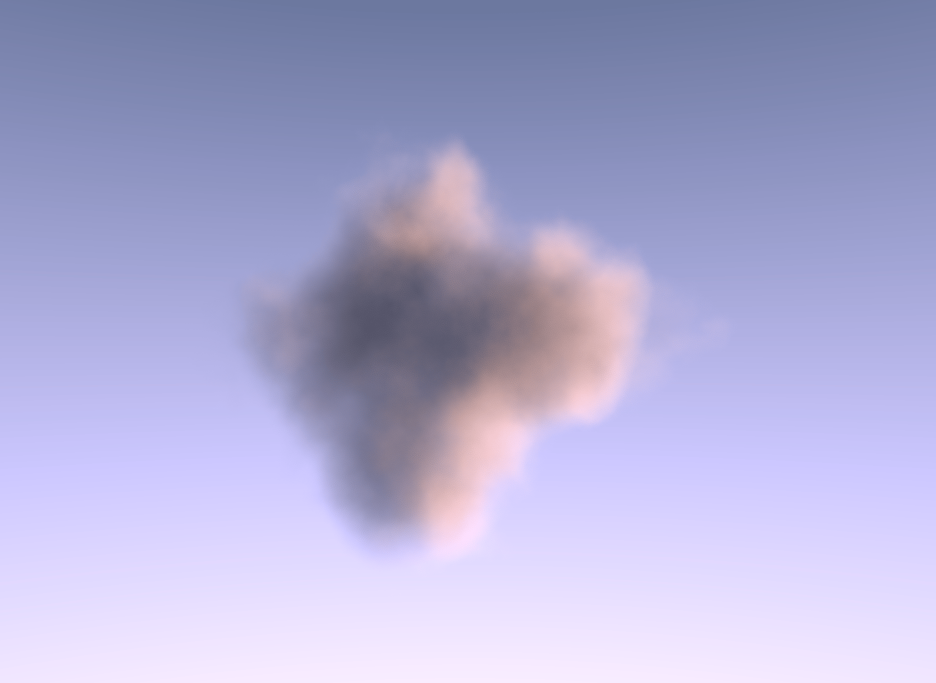
And here's the demo showcasing our blue noise dithering in action giving us a softer cloud ⛅:
Upscaling with Bicubic filtering
This second improvement recommended by @N8Programs aims to fix some remaining noise artifacts that remain following the introduction of the blue noise dithering to our raymarched scene.
Bicubic filtering is used in upscaling and allows smoothing out some noise patterns while retaining details by calculating the value of a new pixel by considering 16 neighboring pixels through a cubic polynomial (Sources).
I was lucky to find an implementation of bicubic filtering on Shadertoy made by N8Programs himself! Applying it directly to our existing work however, is not that straightforward. We have to add this improvement as its own step or pass in the rendering process, almost as a post-processing effect.
I introduced an easy way to build this kind of pipeline in my article titled Beautiful and mind-bending effects with WebGL Render Targets where I showcase how you can use Frame Buffer Objects (FBO) to apply some post-processing effects on an entire scene which we can use for this use case:
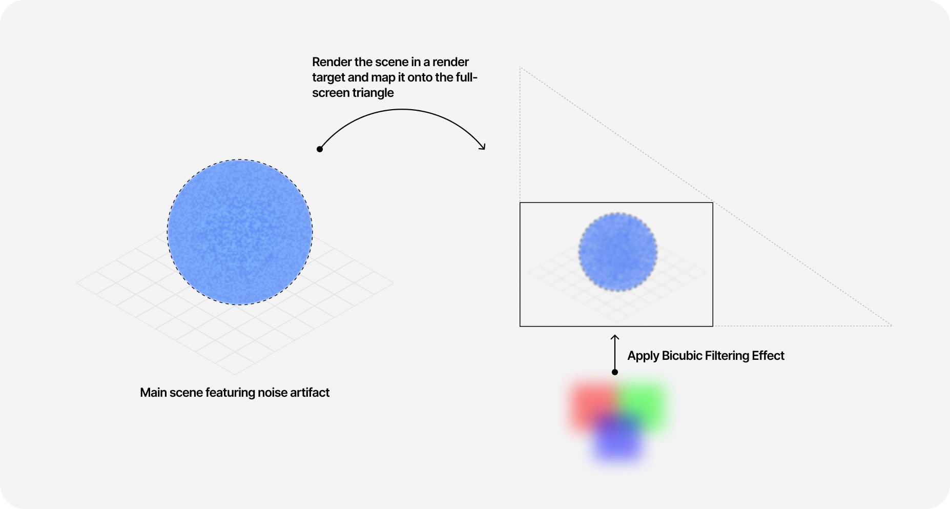
- We render our main raymarched canvas in a portal.
- The default scene only contains a fullscreen triangle.
- We render our main scene in a render target.
- We pass the texture of the main scene's render target as a uniform of our bicubic filtering material.
- We use the bicubic filtering material as the material for our fullscreen triangle.
- Our bicubic filtering will take our noisy raymarched scene as a texture uniform and output the smoothed out scene.
Here's a quick comparison of our scene before and after applying the bicubic filtering:

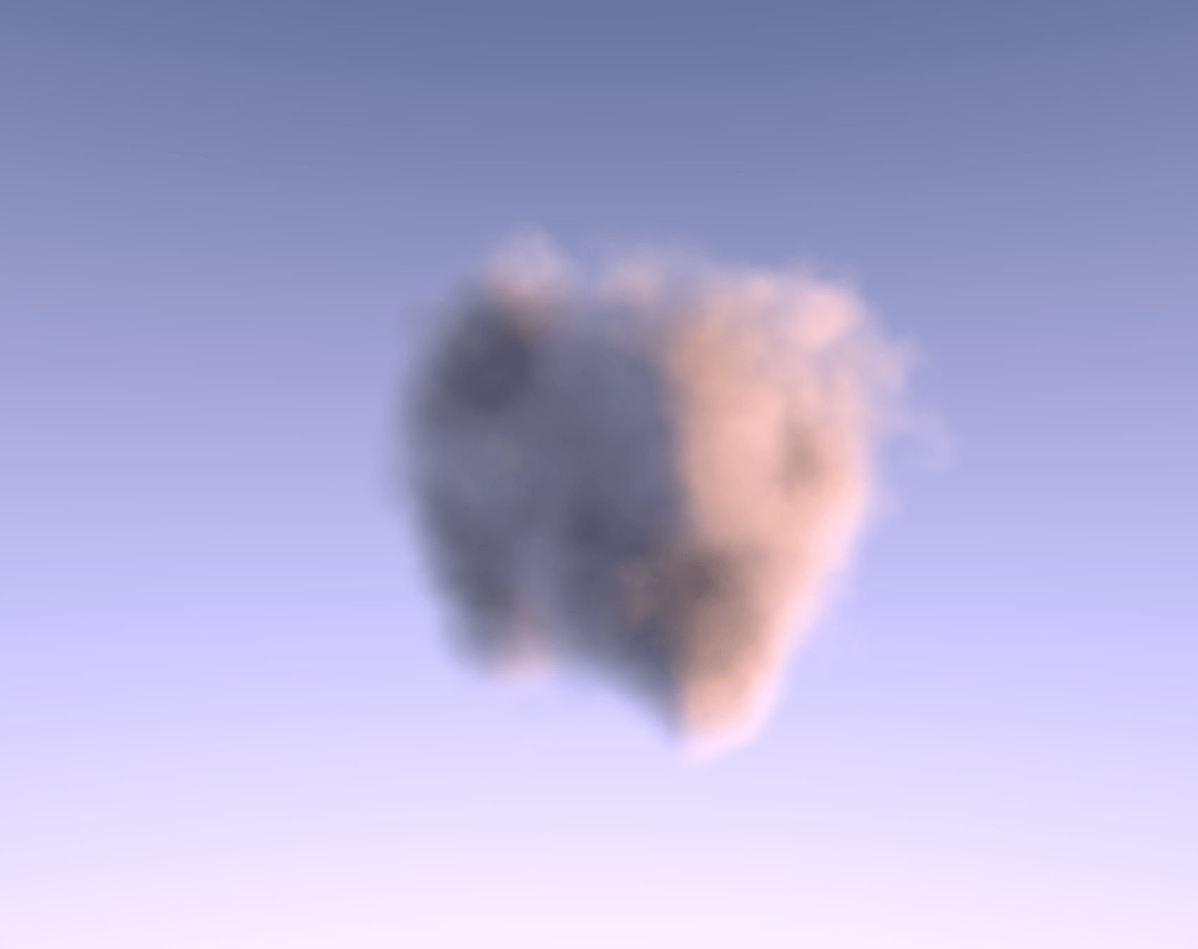
The full implementation is a bit long, and features concepts I already went through in my render target focused blog post, so I invite you to look at it on your own time in the demo below:
Leveraging render targets allowed me to play more with the resolution of the original raymarched scene. You can see a little selector that lets you pick at which resolution we render our raymarched cloud. You can notice that there are not a lot of differences between 1x and 0.5x which is great: we can squeeze more FPS without sacrificing the output quality 🎉.
So far, we've managed to build really beautiful cloudscapes with Volumetric Raymarching using some simple techniques and mixing the right colors. The resulting scenes are satisfying enough and give the illusion of large, dense clouds, but what if we wanted a more realistic output?
I spent quite some time digging through talks, videos, and articles on how game engines solve the problem of physically accurate clouds and all the techniques involved in them. It's been a journey, and I wanted to dedicate this last section to this topic because I find the subject fascinating: from a couple of physical principles of actual real-life clouds, we can render clouds in WebGL using Volumetric Raymarching!
Beer's Law
I already introduced the concept of Beer's Law in my Raymarching blog post as a way to render fog in the distance of a scene. It states that the intensity of light passing through a transparent medium is exponentially related to the distance it travels. The further to the medium light propagates, the more it is being absorbed. The formula for Beer's Law is as follows:
I = I0 * exp(−α * d), where α is the absorption or attenuation coefficient describing how "thick" or "dense" the medium is. In our demos, we'll consider an absorption coefficient of 0.9, although I'd invite you to try different values so you can see the impact of this number on the resulting render.
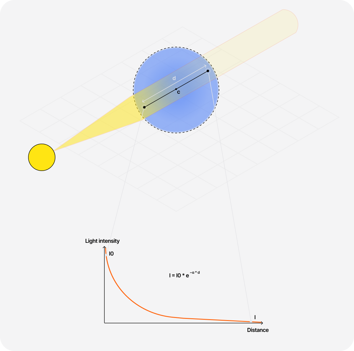
We can use this formula in our GLSL code and modify the Raymarching loop to use it instead of the "hacky" transparency hack we used in the first part:
Using Beer's Law to calculate and return the accumulated light energy going through the cloud
1#define MAX_STEPS 502#define ABSORPTION_COEFFICIENT 0.934//...56float BeersLaw (float dist, float absorption) {7return exp(-dist * absorption);8}910const vec3 SUN_POSITION = vec3(1.0, 0.0, 0.0);11const float MARCH_SIZE = 0.16;1213float raymarch(vec3 rayOrigin, vec3 rayDirection, float offset) {14float depth = 0.0;15depth += MARCH_SIZE * offset;16vec3 p = rayOrigin + depth * rayDirection;17vec3 sunDirection = normalize(SUN_POSITION);1819float totalTransmittance = 1.0;20float lightEnergy = 0.0;2122for (int i = 0; i < MAX_STEPS; i++) {23float density = scene(p);2425if (density > 0.0) {26float transmittance = BeersLaw(density * MARCH_SIZE, ABSORPTION_COEFFICIENT);27float luminance = density;2829totalTransmittance *= transmittance;30lightEnergy += totalTransmittance * luminance;31}3233depth += MARCH_SIZE;34p = rayOrigin + depth * rayDirection;35}3637return lightEnergy;38}
In the code snippet above:
- We gutted the raymarching loop, so it now relies on a more physically based property: Beer's Law.
- We changed the interface of our function: instead of returning a full color, it now returns a
floatrepresenting the amount of light or light energy going through the cloud. - As we march through the volume, we accumulate the obtained
transmittance. The deeper we go, the less light we add. - We return the resulting
lightEnergy
The demo below showcases what using Beers Law yields in our Raymarching loop 👀
The resulting cloud is a bit strange:
- its edges do indeed behave like a cloud
- the center is just a white blob
all of which is, once again, due to the lack of a proper lighting model.
Sampling light
Our new cloud does not interact with light right now. You can try changing the SUN_POSITION vector: the resulting render will remain the same. We not only need a lighting model but also a physically accurate one.
For that, we can try to compute how much light has been absorbed for each sample point of our Raymarching loop by:
- Start a dedicated nested Raymarching loop that goes from the current sample point to the light source (direction of the light)
- Sample the density and apply Beer's Law like we just did
The diagram below illustrates this technique to make it a bit easier to understand:
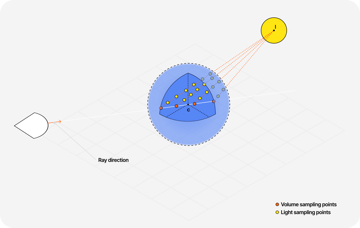
The code snippet below is one of many implementations of this technique. We'll use this one going forward:
Dedicated nested raymarching loop to sample the light received at a given sampled point
1#define MAX_STEPS 502#define MAX_STEPS_LIGHTS 63#define ABSORPTION_COEFFICIENT 0.945//...67const vec3 SUN_POSITION = vec3(1.0, 0.0, 0.0);8const float MARCH_SIZE = 0.16;910float lightmarch(vec3 position, vec3 rayDirection) {11vec3 lightDirection = normalize(SUN_POSITION);12float totalDensity = 0.0;13float marchSize = 0.03;1415for (int step = 0; step < MAX_STEPS_LIGHTS; step++) {16position += lightDirection * marchSize * float(step);1718float lightSample = scene(position, true);19totalDensity += lightSample;20}2122float transmittance = BeersLaw(totalDensity, ABSORPTION_COEFFICIENT);23return transmittance;24}2526float raymarch(vec3 rayOrigin, vec3 rayDirection, float offset) {27float depth = 0.0;28depth += MARCH_SIZE * offset;29vec3 p = rayOrigin + depth * rayDirection;30vec3 sunDirection = normalize(SUN_POSITION);3132float totalTransmittance = 1.0;33float lightEnergy = 0.0;3435for (int i = 0; i < MAX_STEPS; i++) {36float density = scene(p, false);3738// We only draw the density if it's greater than 039if (density > 0.0) {40float lightTransmittance = lightmarch(p, rayDirection);41float luminance = density;4243totalTransmittance *= lightTransmittance;44lightEnergy += totalTransmittance * luminance;45}4647depth += MARCH_SIZE;48p = rayOrigin + depth * rayDirection;49}5051return lightEnergy;52}
Because of this nested loop, the algorithmic complexity of our Raymarching loop just increased, so we'll need to define a relatively low number of steps to sample our light while also calculating a less precise density by reducing the number of Octaves in our FBM to preserve a decent frame-rate (that's one easy win I implemented to avoid dropping too many frames).
All these little tweaks and performance considerations have been taken into account in the demo below:
Anisotropic scattering and phase function
Until now, we assumed that light gets distributed equally in every direction as it propagates through the cloud. In reality, the light gets scattered in different directions with different intensities due to water droplets. This phenomenon is called Anisotropic scattering (vs. Isotropic when light scatters evenly), and to have a realistic cloud, we can try to take this into account within our Raymarching loop.
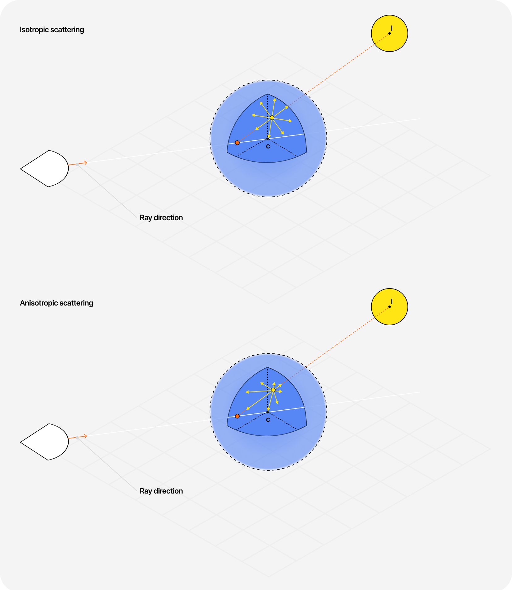
To simulate Anisotropic scattering in our cloud scene for each sampling point for a given light source, we can use a phase function. A common one is the Henyey-Greenstein phase function, which I encountered in pretty much all the examples I could find on physically accurate Volumetric Raymarching.
The GLSL implementation of this phase function looks as follows:
Implementation of the Henyey-Greenstein phase function
1float HenyeyGreenstein(float g, float mu) {2float gg = g * g;3return (1.0 / (4.0 * PI)) * ((1.0 - gg) / pow(1.0 + gg - 2.0 * g * mu, 1.5));4}
We now have to introduce the result of this new function in our Raymarching loop by multiplying it by the density at a given sampled point, and what we obtain is more realistic lighting for our cloud, especially if the light source moves around.
Introducing the Henyey-Greenstein phase function inside our Raymarching loop
1float raymarch(vec3 rayOrigin, vec3 rayDirection, float offset) {2float depth = 0.0;3depth += MARCH_SIZE * offset;4vec3 p = rayOrigin + depth * rayDirection;5vec3 sunDirection = normalize(SUN_POSITION);67float totalTransmittance = 1.0;8float lightEnergy = 0.0;910float phase = HenyeyGreenstein(SCATTERING_ANISO, dot(rayDirection, sunDirection));1112for (int i = 0; i < MAX_STEPS; i++) {13float density = scene(p, false);1415// We only draw the density if it's greater than 016if (density > 0.0) {17float lightTransmittance = lightmarch(p, rayDirection);18float luminance = density * phase;1920totalTransmittance *= lightTransmittance;21lightEnergy += totalTransmittance * luminance;22}2324depth += MARCH_SIZE;25p = rayOrigin + depth * rayDirection;26}2728return lightEnergy29}
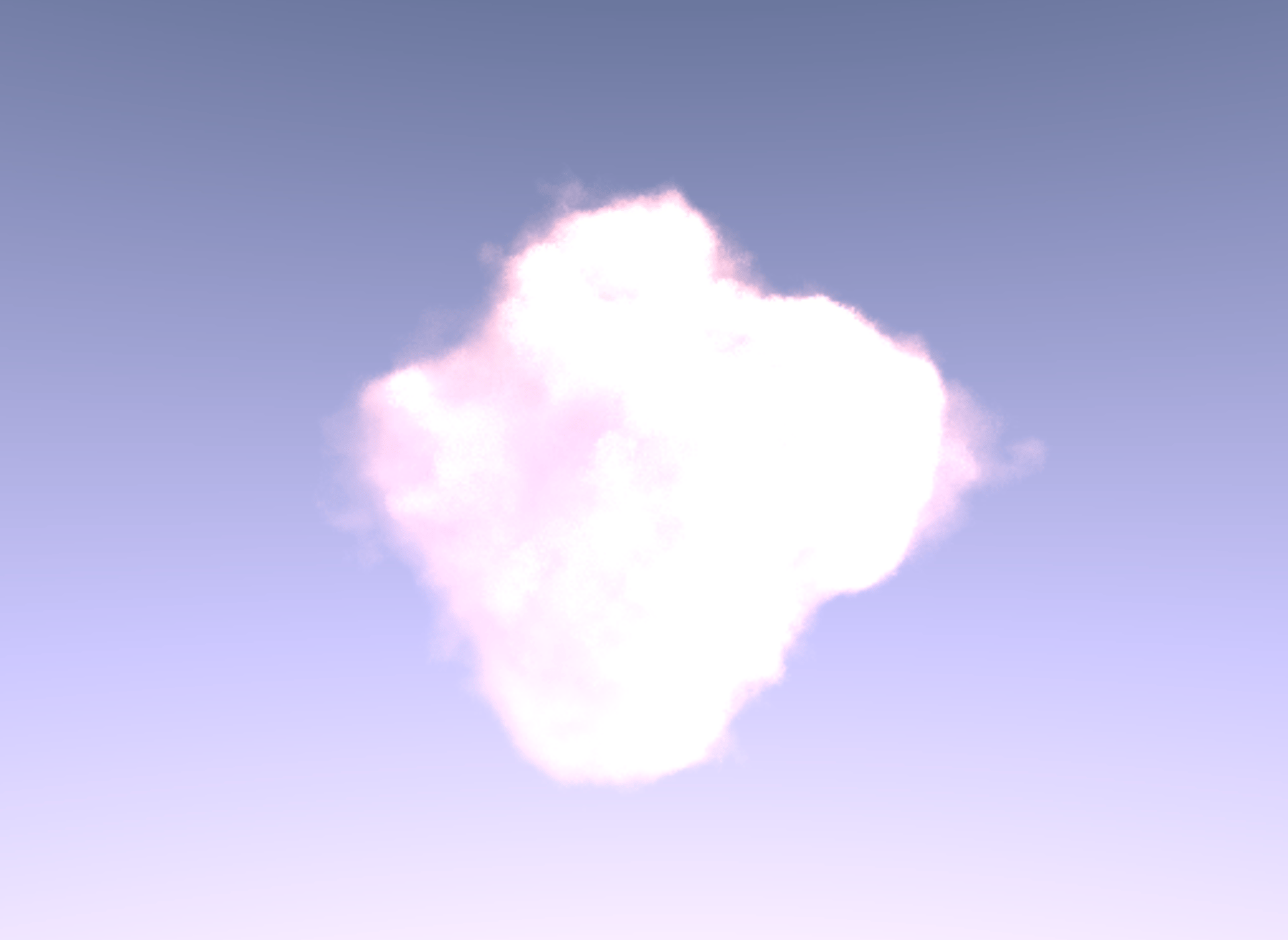
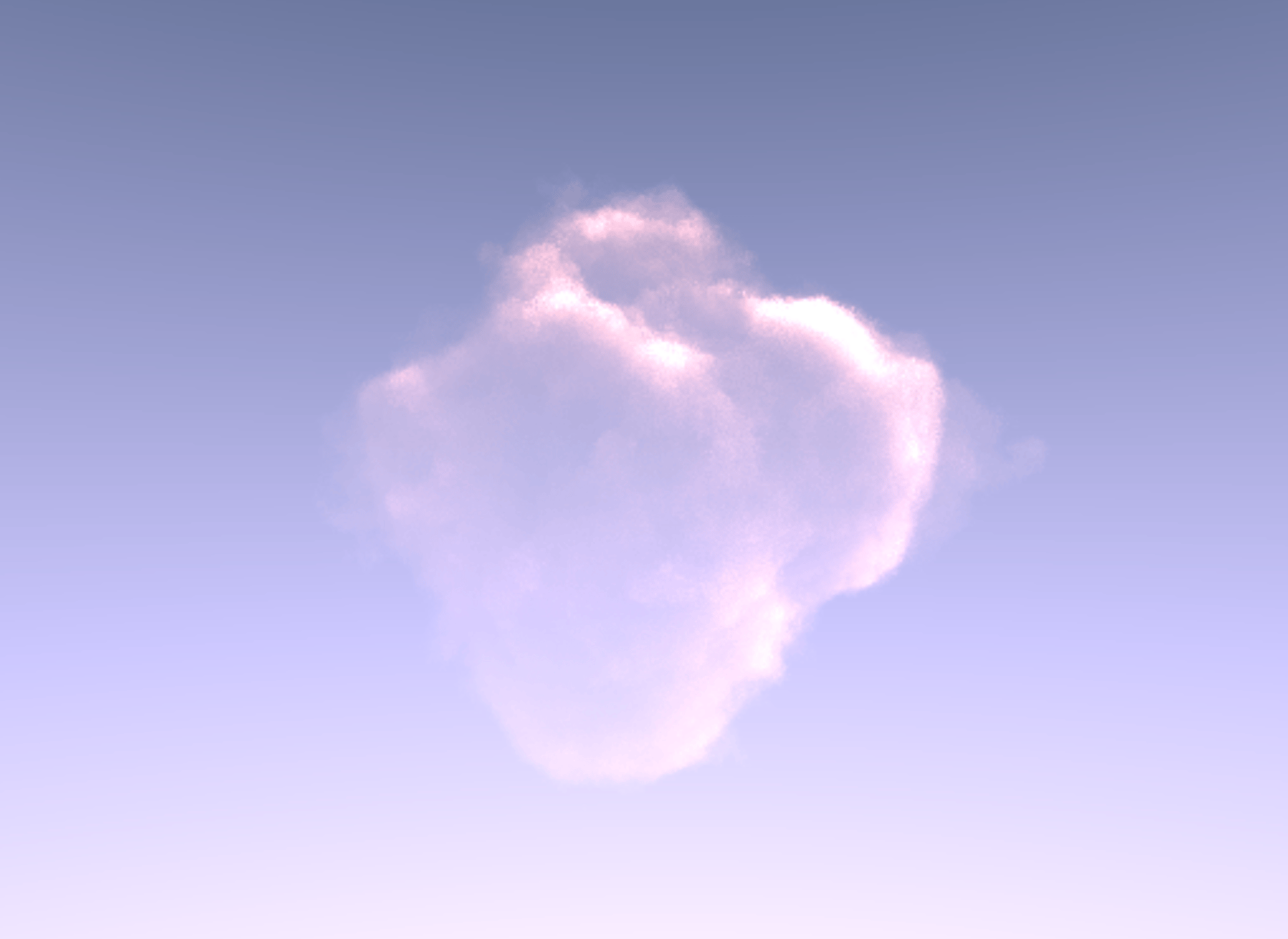
The final demo of this article below showcases our scene with:
- Blue noise dithering
- Bicubic filtering
- Beer's law
- Our more realistic light sampling
- Henyey-Greenstein phase function
The result is looks really good, although I'll admit I had to add an extra value term to my light energy formula so the cloud wouldn't simply "fade away" when dense parts would end up in the shade.
Extra value added to the luminance formula
1float luminance = 0.025 + density * phase;
The need for a hack probably highlights some issues with my code, most likely due to how I use the resulting light energy value returned by the Raymarching loop or an absorption coefficient that's a bit too high. Not sure. If you find any blatantly wrong assumptions in my code, please let me know so I can make the necessary edits.
Some other optimizations are possible to make the cloud look fluffier and denser, like using the Beer's Powder approximation (page 64), but it was mentioned to me that those are just used for aesthetic reasons and are not actually physically based (I also honestly couldn't figure out how to apply it without altering significantly my MAX_STEPS, MAX_STEPS_LIGHTS, and marchSize variables 😅 and the result was still not great).
@MaximeHeckel Note that beer-powder is a non-physical approximation. Maybe see: https://t.co/LlHxW5x5sb
We learned several ways to render cloud-like volumes with Raymarching throughout this article, and considering that a few weeks prior to that, I wasn't even able to wrap my head around the concept of Volumetric Raymarching, I'm happy with the result and proud of myself given how complex and daunting this subject can be. I was also pleasantly surprised by the ability to apply some physics principles and port techniques commonly used in triple-A video game productions to WebGL to achieve realistic looking clouds.
With that, I'm excited to attempt combining raymarched clouds with terrain, like the ones introduced in my Raymarching article, or even more complex challenges like rendering a planet with realistic atmospheric scattering. Another idea I had was to build a raymarched galaxy; since we can simplify it to a massive cloud in space and that some of the physics principles introduced in this article should still apply and yield beautiful renders.
I hope this article will inspire you in your own Raymarching endeavors and that it helped make this seemingly hard-to-grasp concept of Volumetric rendering a bit more welcoming 🙂.