Shading Motion
If you are a long-time reader of this blog, you may have noticed that many of my recent explorations related to graphics programming topics involves some flavor of screen-space shaders. They are incredibly versatile, as we’ve seen through the many effects we’ve studied, ranging from simple pixel manipulation, such as paint or halftone, to more advanced use cases, such as volumetric lighting or atmospheric scattering. Yet, all have one thing in common here. They all treat the underlying image, or frame, as a spatial medium: sampling color, luminance, depth, and neighboring pixels, and use it as the main input for the effect.
This made me wonder: what if, instead, we used motion within the scene as the input to our effects?
I was eager to find a way to extract motion and explore the many ways we could visually interpret it with shaders, even more so after seeing friends experiment with motion-based effects such as blob tracking and optical flow in tools like TouchDesigner. The list of things I wanted to try out and build only grew longer as I dug deeper into this topic, finding novel solutions to edge cases I was encountering or stumbling upon new visuals I wanted to recreate. This new temporal input kept me tinkering creatively for the better part of two months now.
My goal for this article is to introduce you to motion as a new creative medium and explore several ways of representing it with shaders, or simply put, “how to shade motion”, hence the title. Using WebGPU compute shaders, we’ll build a small pipeline to extract motion through frame differencing and encode it into masks and velocity maps. We’ll use those as foundations for a series of effects ranging from simple trails to blob tracking, directional effects, and motion blur with object smearing, each bringing its own set of challenges and new interesting shading techniques that I’m excited to finally share with you.
Unlike luminance or depth, motion is not available straight out of the box for us to sample from a single frame of our scene. Before we can process it or stylize it with a shader, we first need to make it visible.
For this section, our goal is straightforward: we need to establish a pipeline that identifies which parts of the frame change and maps the magnitude of the motion to a luminance texture. The brighter the pixel appears at a given location, the more movement is detected at this position. This will give us a simple representation of motion that we can store, process, and eventually use as the backbone of other effects.
Comparing frames
To produce the luminance map on which our entire pipeline will rest, we’ll first start with the simplest possible approach: comparing the current frame with the previous one. We need at least two points in time, or in this case, two frames, to tell us about what is moving in the scene. By converting both frames to grayscale, subtracting one from the other, and taking the absolute value, we can obtain a grayscale image representing the magnitude of the change for each pixel.
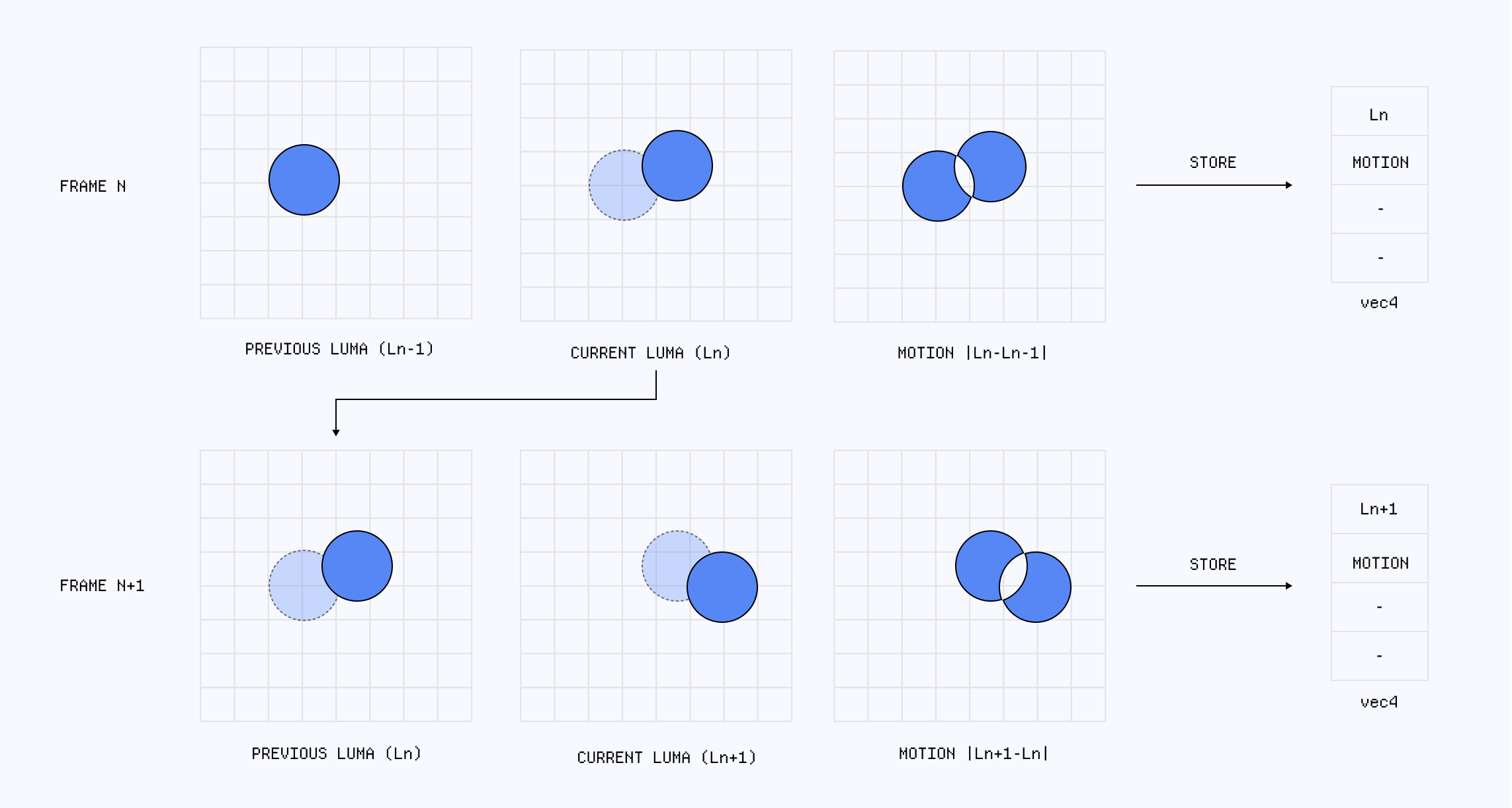
- First, we need access to the current scene and the luma stored during the previous frame.
1let currentColor = textureLoad(videoTexture, videoCoord, 0).rgb;2let currentLuminance = dot(currentColor, vec3f(0.299, 0.587, 0.114));3let previousState = textureLoad(stateReadTexture, vec2i(coord), 0);
- We can then calculate the difference between the frames.
1let difference = abs(currentLuminance - previousState.r);
- We apply a threshold to filter out insignificant changes and produce the motion amount.
1let motionAmount = smoothstep(2motionThreshold,3motionThreshold * 4.0,4difference5);
- We store that value as a grayscale motion mask for subsequent passes/effects.
1textureStore(2stateWriteTexture,3vec2i(coord),4vec4f(currentLuminance, motionAmount, 0.0, 1.0)5);
This method is called frame differencing, and it’s one of the simplest ways to estimate motion from a sequence of images. In my experiments, I used it to extract motion over 3D scenes, videos, or even webcam streams. It does a pretty decent job at giving you a result that you can work with. You can even apply a threshold, as featured in the code example above, to remove noise or subtle movements that may pollute the resulting texture. The widget below showcases this method applied over a video.
While this gives us a luminance map of the motion, which is what we wanted, the output may feel a bit disappointing at first glance. The resulting image is flickering, and the motion is not smooth, which, as you can imagine, may be detrimental to the quality of our effect. Luckily for us, there are a few things we can do about that.
Smooting out the motion
To compensate for the defects of our very simple motion detection process, we can reuse a technique I’ve mentioned in several blog posts: accumulating the previous state and letting it fade over time through temporal decay 1.
Doing so would result in our motion appearing more continuous over time while also leaving a trail from the fading accumulated frames, which we’ll also be able to stylize as we see fit in later examples. Instead of returning the raw threshold mask directly, we need to:
- Retrieve the trail accumulated in the previous frame.
- Multiply it by a
decayvalue to gradually reduce its intensity. - Combine the decayed mask with the newly detected motion.
- Store both the raw motion and its accumulated trail for subsequent passes.
- Swap the trail textures so that the previous trail becomes the result on the next frame.
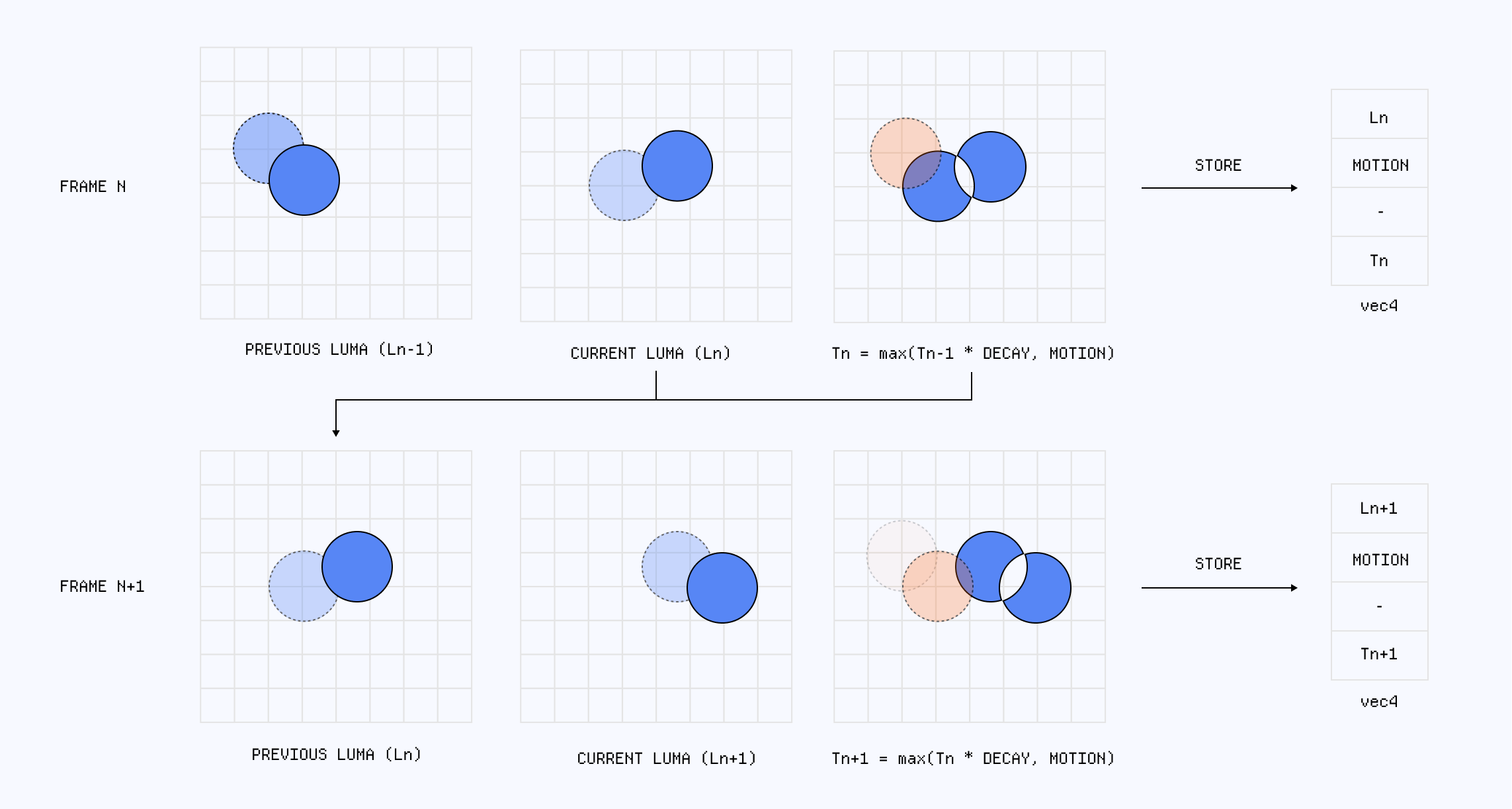
Introducing a decay to generate a trail from the motion
1let decayedTrail = max(previousState.g * trailDecay - 0.025, 0.0);2let motionTrail = max(decayedTrail, motionAmount);34textureStore(5stateWriteTexture,6vec2i(coord),7vec4f(currentLuminance, motionTrail, 0.0, 1.0)8);
This gives us the decay as an extra tool in our belt to tweak the motion mask to our liking:
- The smaller the decay, the faster the accumulated texture will fade out.
- The larger, the longer it will remain on screen, leaving semi-permanent long trails on the canvas.
As for which setting I recommend, it really depends on your input image. For scenes featuring slow movements with a high amplitude, I’d increase the motionThreshold, and keep the decay rate below 0.75. For the ones featuring tiny, subtle motion, I’d give more weight to the trail, as otherwise the surface area where our shader will apply its effect will remain too small to be visible. The widget below showcases a version of the previous mask, but this time with decay.
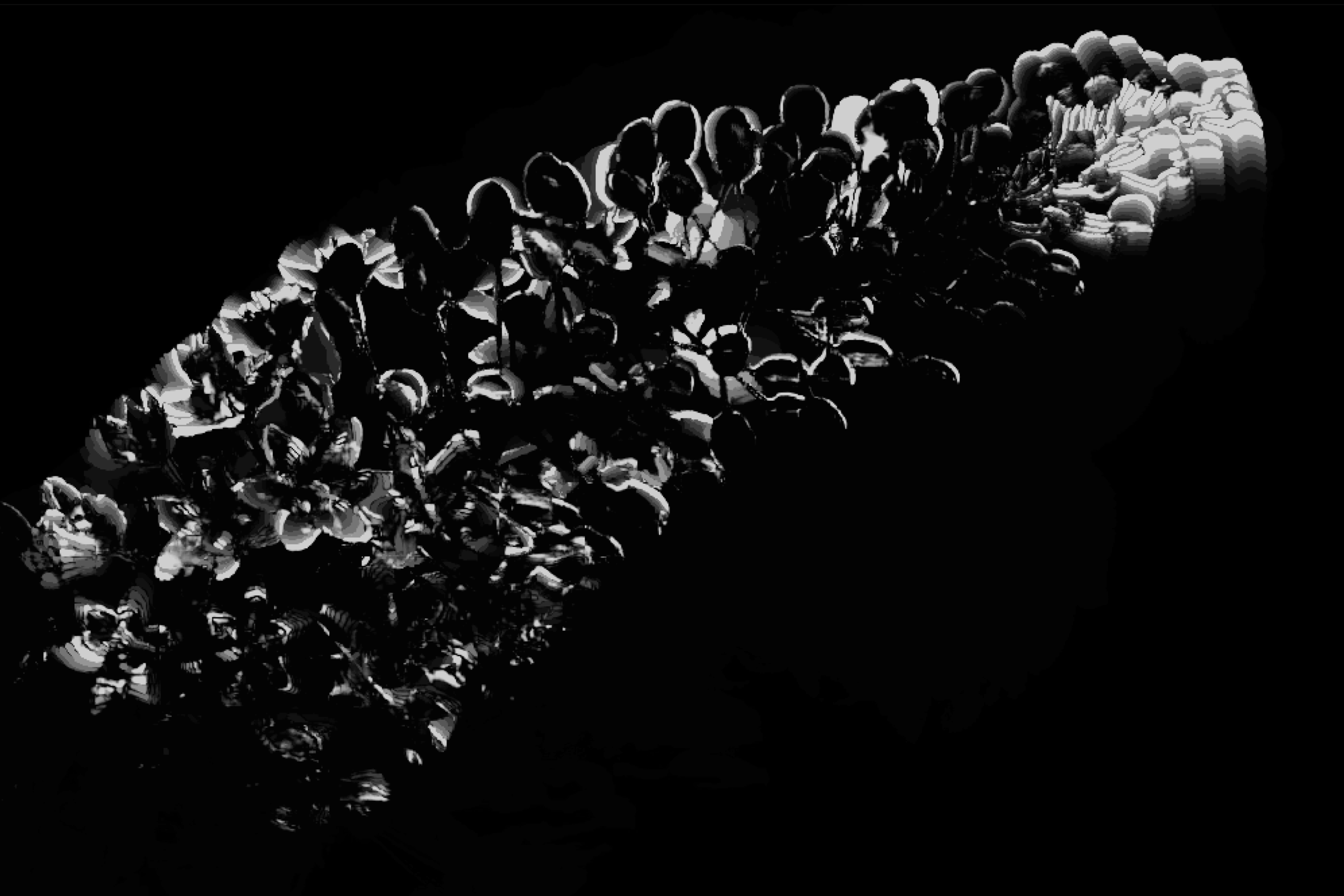
As you can see, this version is a lot more pleasing to the eye and gives us more luminance pixels to work with. With this, we finally have a decent motion mask that will serve as input to the subsequent post-processing passes we will build to stylize the motion.
Stylizing the motion
We can now start putting our motion mask to work. First, we need a way to build the motion mask texture on every frame. This is a task we need to perform independently for every pixel, which is something we can handle in a compute shader.
Each invocation of the compute shader can process one pixel: sample its current and previous luminance values, compute their difference, update the decayed trail, and write the results to a storage texture, as we showcased in the code snippets before this section. Moreover, it will also help us make a clear distinction between:
- The compute stage of our effect, which prepares our data/textures.
- The render stage, which will focus on using those computed textures for the final render.
For a React Three Fiber scene, I like to organize my compute shader as follows 2
Compute shader to compute the motion of a scene
1const createComputeNodes = ({2detectionHeight,3detectionWidth,4resources,5shaderUniforms,6}) => {7const computeMotionMask = wgslFn(8// Motion mask compute shader code goes here.9);1011const createComputeNode = (readIndex, writeIndex) =>12computeMotionMask({13hasPreviousFrame: shaderUniforms.hasPreviousFrame,14index: instanceIndex,15motionThreshold: shaderUniforms.motionThreshold,16stateReadTexture: texture(resources.stateTextures[readIndex]),17stateWriteTexture: storageTexture(18resources.stateTextures[writeIndex],19).toWriteOnly(),20trailDecay: shaderUniforms.trailDecay,21}).compute(detectionWidth * detectionHeight, [8]);2223// We use separate read and write textures for broader WebGPU support.24// These two nodes let each frame swap which texture holds25// the previous state.26return [27createComputeNode(0, 1), // Read A, write B.28createComputeNode(1, 0), // Read B, write A.29];30};3132const hasPreviousFrameRef = useRef(false);33const currentBufferIndexRef = useRef(0);3435const shaderUniforms = useMemo(36() => ({37hasPreviousFrame: uniform(false),38motionThreshold: uniform(0.1),39trailDecay: uniform(0.98),40}),41[],42);4344const computeNodes = useMemo(45() =>46createComputeNodes({47detectionHeight,48detectionWidth,49resources,50shaderUniforms,51}),52[detectionHeight, detectionWidth, resources, shaderUniforms],53);5455useFrame(() => {56const computeIndex = currentBufferIndexRef.current;5758// Skip motion detection until a previous frame has been stored.59shaderUniforms.hasPreviousFrame.value = hasPreviousFrameRef.current;6061// Compare both frames and write the new luminance and motion trail.62gl.compute(computeNodes[computeIndex]);6364hasPreviousFrameRef.current = true;6566// Use the texture we just wrote as the previous state on the next frame.67currentBufferIndexRef.current = 1 - computeIndex;68});
With that in place, we have a compute shader running on every frame in our browser computing our motion mask. The resulting texture can now be passed to the render pipeline and used, for example, as input for a post-processing effect.
Rendering the detected motion as an effect
1const outputNode = Fn(() => {2const motionMask = texture(trailTexture).g;3const cool = vec3(0.0, 0.5, 2.0);4const hot = vec3(1.0, 0.35, 0.5);5const heatColor = mix(cool, hot, motionMask);67return vec4(heatColor.mul(motionMask), 1.0);8})();910postProcessing.outputNode = outputNode;11postProcessing.render();
The code snippet above is a simple example of some sort of heatmap effect where we color the trailtexture based on its intensity:
- The brighter the detected motion, the more orange it will appear.
- The dimmer, the less motion there is, and thus the related pixels will tend towards blue.
We can see this effect at work in the demo below, built on top of the decayed motion mask demo shown earlier:
This is the moment where the possibilities become endless, as you have total freedom to interpret the motion mask as you please. Here we did a heatmap, but you might as well render the motion as a pixelated trail, or split the screen in half to render the stylized detected motion on one half while rendering the original input in the other, as I did below.
The beauty of this simple pipeline is that it compounds elegantly with concepts and techniques we’ve seen in other post-processing-related blog posts, such as Post-processing as a Creative Medium, since, after all, the only thing we really did in this first pass was transform the motion into luminance. The playground below features the full compute and render phase with an example of a motion effect, a recreation of my demo titled “data stream” applied on top of a 3D scene
While our motion mask tells us where individual pixels changed from one frame to another, it does not highlight the larger moving elements they belong to. Grouping those into coherent regions would unlock a new kind of visual for our render pipeline, allowing us to shade the image based on clusters of motion rather than discrete pixels.
This is the main idea behind Blob Tracking: an effect that overlays connected motion areas with boxes, crosshairs, connecting segments, or any other shapes we may choose. My definition may sound vague, but I’m sure you’ve encountered this visual language before, especially among creators in the TouchDesigner community. Just in case, here’s an example:
Often, these geometric shapes and data-heavy overlays characteristic of this effect are found over nature/cityscape time-lapses or macro footage of plants growing and blooming. Another great example of contrasting aesthetic. I did the same for my own take on this effect:


blob tracking effect built with WebGPU had fun playing with motion-based effects alongside sound over the past few weeks :) https://t.co/bp2KFkaG8U https://t.co/cgiuaZCR9n
In this section, we will walk through the process of reimplementing this effect in WebGPU, on top of the pipeline we built in the first part of this article. The goal would be to approach the visuals from TouchDesigners while remaining relatively performant.
Detecting motion blobs
Our motion mask already has all the necessary information we need to find blobs. The only thing we need to do now is to structure that data into a collection of motion clusters. To do so, we will define a data structure composed of:
{x,y}coordinates for the center of a given blob- a size
s - a confidence
c, a value representing whether a given slot is valid/active
With this data structure in mind, we should have all the information needed to draw the blobs. However, we still need to translate our motion mask to extract and store the data, and for that we will use another compute shader to run a blob detection algorithm. The steps of this algorithm are broken down and illustrated below:
This algorithm works on a predefined number of “blob slots”, i.e., a maximum number of blob items we will draw on screen. This example features 5, but I went up to 12 in my own demos. For each of these blob slots we:
- Choose a search center: we start from seeds distributed across the image. If the blob already has a valid position from a previous frame, we use that position instead.
1let previousState = blobStateBuffer[index];2let wasActive = previousState.w > 0.03;3let slot = f32(index);4let seed = vec2f(5fract(slot * 0.61803398875 + 0.13),6fract(slot * 0.38196601125 + 0.31)7);8let probeCenter = select(seed, previousState.xy, wasActive);9let searchRadius = select(0.45, 0.28, wasActive);
- Sample a
5 x 5region: we place 25 evenly spaced samples across a square centered on the search position, and read the motion strength at each point.
1for (var sampleIndex = 0u; sampleIndex < 25u; sampleIndex++) {2let sx = f32(sampleIndex % 5u) / 4.0 - 0.5;3let sy = f32(sampleIndex / 5u) / 4.0 - 0.5;4let sampleUv = clamp(5probeCenter + vec2f(sx, sy) * searchRadius,6vec2f(0.0),7vec2f(1.0)8);9let sampleCoord = clamp(10vec2i(sampleUv * vec2f(dimensions)),11vec2i(0),12vec2i(dimensions) - vec2i(1)13);14let motionSample = textureLoad(stateTexture, sampleCoord, 0);1516// Weight and accumulate this sample next.17}
- Weight each sample by motion, distance, and exclusion: we give more influence to samples with stronger motion and samples closer to the center. If blobs are already claimed by an earlier slot, we reduce their weight to prevent slots from converging to the same regions.
1// Running totals across all 25 samples:2// - weightSum normalizes the final center.3// - weightedCenter accumulates weighted UVs (X = U, Y = V).4// - weightedSecondMoment accumulates weighted U² and V² to estimate spread i.e. the variance.5// Needed because variance = mean(position²) - mean(position)²6var weightSum = 0.0;7var weightedCenter = vec2f(0.0);8var weightedSecondMoment = vec2f(0.0);910// For each point in the 5 x 5 sample:11// stateTexture stores current luminance in R, raw motion in G,12// nothing in B, and the accumulated motion trail in A.13// Favor the current motion while retaining a little of its recent history.14let trackedMotion = motionSample.g * 0.8 + motionSample.a * 0.2;1516// sx and sy are the sample's offset from the probe center.17// Samples near that center receive more influence.18let falloff = max(0.0, 1.0 - length(vec2f(sx, sy)) * 1.25);1920// Start with no exclusion, i.e. full weight factor21var exclusion = 1.0;2223for (var otherIndex = 0u; otherIndex < index; otherIndex++) {24// Each blob stores its center in XY, size in Z, and confidence in W.25let otherBlob = blobStateBuffer[otherIndex];2627if (otherBlob.w > 0.04) {28// Reduce this sample's influence when it is close to a blob29// already claimed by an earlier slot.30exclusion *= smoothstep(310.035,320.13,33length(sampleUv - otherBlob.xy)34);35}36}3738// Combine motion strength, distance falloff, and exclusion into one weight.39let weight = trackedMotion * falloff * exclusion;4041// Accumulate the total weight, weighted position, and weighted squared position.42weightSum += weight;43weightedCenter += sampleUv * weight;44weightedSecondMoment += sampleUv * sampleUv * weight;
- Calculate the weighted center.
1let center = weightedCenter / max(weightSum, 0.0001);
- Get the size from the weighted variance.
1let variance = max(2weightedSecondMoment / max(weightSum, 0.0001) - center * center,3vec2f(0.0)4);5let size = clamp(6sqrt(max(variance.x, variance.y)) * 0.85,70.02,80.829);
- Store the result in an array buffer.
1blobStateBuffer[index] = vec4f(center, size, confidence);
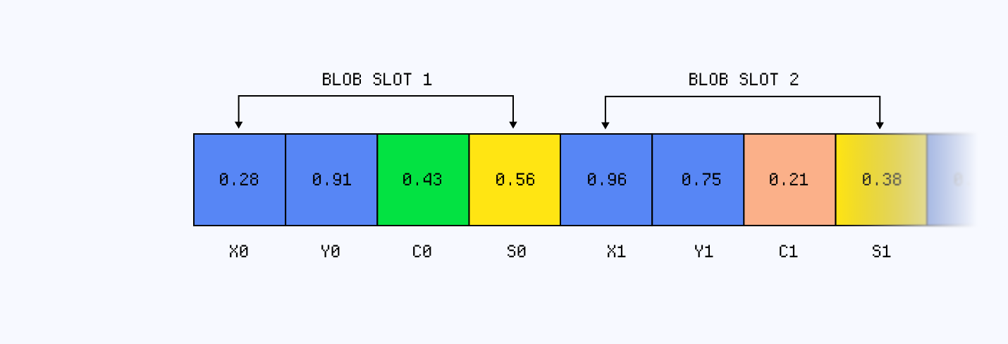
The resulting storage buffer is tiny. Each of the 12 blob slots stores four 32-bit floats for a total of just 12 * 4 floats * 4 bytes (32 bits / 8 bits = 4 bytes) = 192 bytes.
Through this process, we’ve transformed the motion mask into a compact buffer representing our detected blobs. We can now send that buffer to the rest of the pipeline, finally getting to the fun part: drawing the blobs.
Drawing blobs
With this buffer at the ready, we can start thinking about how to draw the visuals that will represent our blobs in our final effect. Once again, the sky is the limit here; the only thing that really matters is that the resulting overlay pleases you. For this post, I’m just going to cover the classic types of visuals and, more importantly, the method I used to render them.
To draw shapes such as squares, circles, crosshairs, or segments, we will have to rely on Signed Distance Functions 3, SDF, to which we will pass from our buffer:
- The center coordinates
{x, y}to position the shape on screen. - The size
sto scale it.
Below are a couple of examples of shapes and their corresponding SDFs that can serve as a reminder, or just a light introduction:
1float sdBox(vec2 p, vec2 b) {2vec2 d = abs(p) - b;34return length(max(d, 0.0)) + min(max(d.x, d.y), 0.0);5}67float shapeDistance(vec2 p) {8return abs(sdBox(p, vec2(0.5, 0.5)));9}
To use them in our effect, we will have to:
- Read and loop through our buffer to retrieve the blob slot data.
1const boxMask = float(0.0).toVar();23for (let i = 0; i < maxBlobs; i++) {4// XY = center, Z = size, W = confidence.5const blob = resources.blobStateBuffer.element(i);6const center = vec2(blob.x.mul(targetAspect), blob.y);78// Draw the current blob...9}
- Convert our size to
halfSize, since our SDFs measure the shape from its center to its edges. Thus, we have to divide the size by two.
1const halfSize = vec2(blob.z).mul(0.5);2const distanceToBox = boxSdf(drawUv.sub(center), halfSize);
- Only draw the blob when we’re above a certain threshold of confidence. Plus, we also do not forget to antialias the output.
1const active = blob.w.greaterThan(0.04).toFloat();2const edgeWidth = fwidth(distanceToBox).mul(2.5);3const box = smoothstep(0.0, edgeWidth, abs(distanceToBox))4.oneMinus()5.mul(active);67boxMask.assign(max(boxMask, box));
Rendering this effect on top of our scene, whether it is a simple video or a 3D scene, should result in a series of boxes, circles, or crosshairs, depending on which SDF you picked, moving across the screen over the main motion clusters. The playground below features the full code we just went through for our compute and render pipelines:
Now, some blob-tracking examples also feature segments connecting the centers of different blobs on screen. How should we go about that? With SDFs once again!
To draw a segment, we find the point on the line closest to the current pixel and measure the distance between them. Pixels close enough to the line become visible, while those farther away fade out smoothly using smoothstep. For more complex curved segments, the principle remains the same, except that we first need to evaluate a Bézier curve 4 at that position before measuring the distance. The widget below shows both segment types and their corresponding SDFs.
1float sdSegment(vec2 p, vec2 a, vec2 b) {2vec2 pa = p - a;3vec2 ba = b - a;45float segmentLengthSq = max(dot(ba, ba), 0.0001);6float projection = dot(pa, ba) / segmentLengthSq;7float t = clamp(projection, 0.0, 1.0);89vec2 closestPoint = a * (1.0 - t) + b * t;1011return smoothstep(0.0, uThickness, length(p - closestPoint));12}1314float shapeDistance(vec2 p) {15vec2 start = vec2(0.1, 0.9) * 2.0 - 1.0;16vec2 end = vec2(0.9, 0.1) * 2.0 - 1.0;1718return sdSegment(p, start, end);19}
As to how to include them in our effect, I chose to do something pretty stupidly simple: link one blob to the next in the order we read them in the buffer:
Linking blob centers
1const nextBlob = resources.blobStateBuffer.element(2(i + 1) % maxBlobs,3);4const nextActive = nextBlob.w.greaterThan(0.04).toFloat();5const nextCenter = vec2(nextBlob.x.mul(targetAspect), nextBlob.y);67const straightPoint = straightSegmentPoint(drawUv, center, nextCenter);8const curvedPoint = curvedSegmentPoint(drawUv, center, nextCenter);9const segmentPoint = mix(straightPoint, curvedPoint, segmentType);1011const distanceToSegment = distance(drawUv, segmentPoint);12const line = smoothstep(130.0,140.002,15distanceToSegment,16)17.oneMinus()18.mul(active)19.mul(nextActive);
This simple hack creates an organic chain of connected shapes that follows the blobs across the screen.
Using blobs as masks
Blob Tracking, as an effect, is loosely defined; some creators will call it a day once they reach the point where we are now, while others will build on it by adding text, morphing shapes, or other visual elements. One simple addition I personally like a lot is to use the shapes as masks to render a custom shader within them.
Using the SDF we defined earlier, each blob can generate a black-and-white mask:
1.0for pixels inside a blob’s shape0.0for pixels outside it
Defining a mask from our blobs
1const fillMask = float(0.0).toVar();23for (let i = 0; i < maxBlobs; i++) {4const blob = resources.blobStateBuffer.element(i);5const active = blob.w.greaterThan(0.04).toFloat();6const center = vec2(blob.x.mul(targetAspect), blob.y);7const halfSize = vec2(blob.z).mul(0.75);8const distanceToBox = boxSdf(drawUv.sub(center), halfSize);9const edgeWidth = fwidth(distanceToBox).mul(2.5);1011// The filled SDF is 1 inside the box and 0 outside.12const fill = smoothstep(0.0, edgeWidth, distanceToBox)13.oneMinus()14.mul(active);1516fillMask.assign(max(fillMask, fill));17}
With this, we can isolate the pixels inside from the outside ones and choose to apply a shader on either.
Applying an effect inside our blob boxes
1const effectColor = thermalEffect(videoColor);23// Keep the video outside the blobs and reveal the effect inside them.4color.assign(mix(videoColor, effectColor, fillMask));
The playground below showcases this flavor of blob tracking built on top of the previously implemented blob shapes and segments, with the option for you to apply the shader in or out of the boxes.
We now have a convincing blob-tracking effect implemented in WebGPU. We used compute shaders to locate the blobs in each frame from a motion mask, and overlay a series of shapes and effects on top of them. From here, I encourage you to keep experimenting and use what we built as a starting point for your own ideas.
The previous section featured a practical example of using detected motion beyond simple masking. As is, the motion masking texture encodes where clusters of motion beyond a certain threshold are located, but it cannot tell us in which direction they are moving. In this part, we’re going to work towards extracting that information from the motion mask and building an optical flow-inspired effect where we’ll draw a field of arrows/vectors over the scene representing the direction of the detected movement.
@poetengineer__ has a great example of this effect among her many visual experiments. Hers relies on OpenCV, which I’d recommend using if you want accuracy. Our goal here, however, is to have an additional shader input for creative purposes rather than production-grade computer vision.

Extracting the direction of motion
Our motion mask as of now represents motion intensity in a grayscale texture as luminance. What we need here instead is a way to represent the motion vector field. To do so, we can compare each pixel in the current frame with neighboring pixels in the previous frame to estimate the direction of movement, and represent the direction as distinct colors in the resulting texture:
- Red → the luma at the current frame
- Green above
0.5→ movement toward the right - Green below
0.5→ movement toward the left - Blue above
0.5→ movement upward - Blue below
0.5→ movement downward - Alpha → persistence of the motion trail
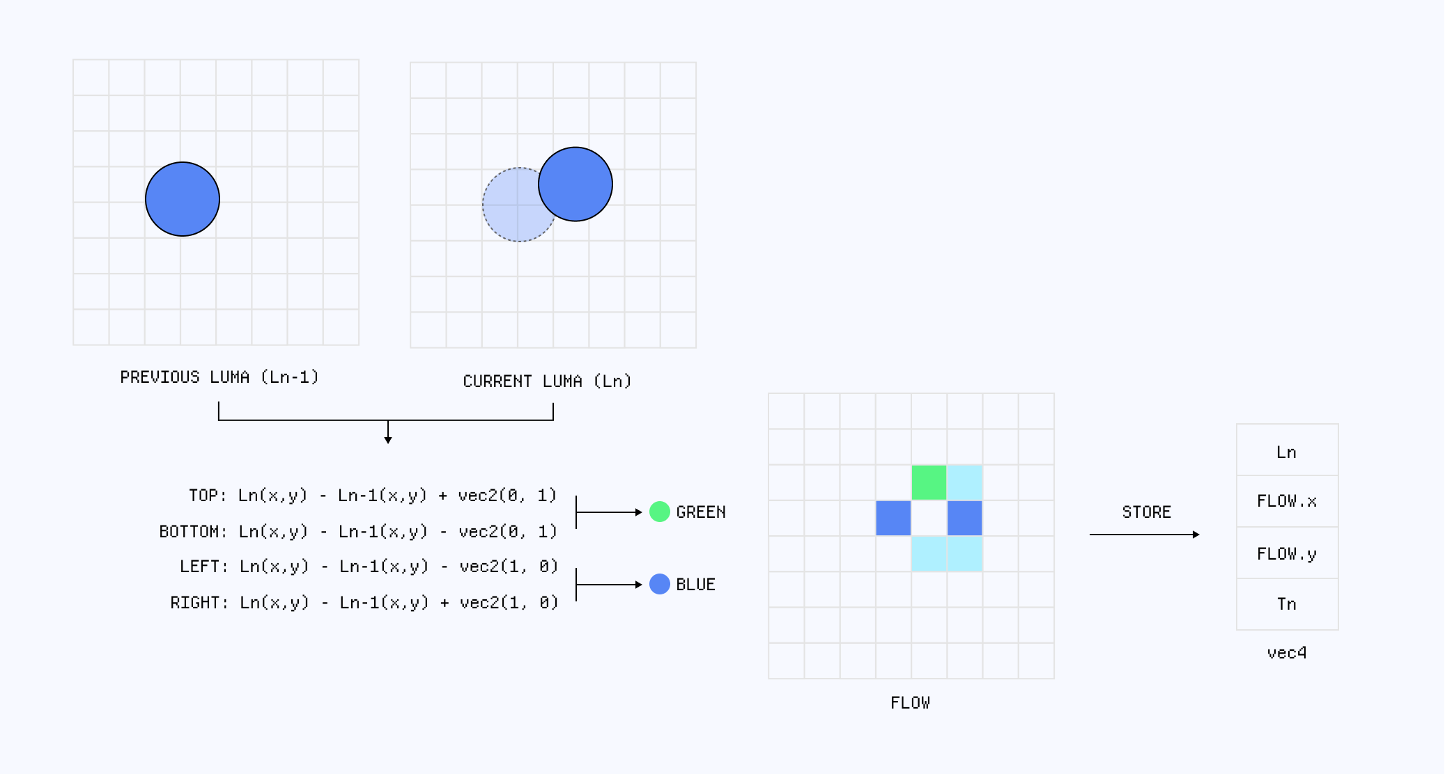
The code snippet below shows the updated logic of our first compute shader and the updated resulting texture we write to:
Updated compute shader computing the flow of motion
1let leftCoord = clamp(2vec2i(coord) - vec2i(1, 0),3vec2i(0),4vec2i(dimensions) - vec2i(1)5);6let rightCoord = clamp(7vec2i(coord) + vec2i(1, 0),8vec2i(0),9vec2i(dimensions) - vec2i(1)10);11let upCoord = clamp(12vec2i(coord) - vec2i(0, 1),13vec2i(0),14vec2i(dimensions) - vec2i(1)15);16let downCoord = clamp(17vec2i(coord) + vec2i(0, 1),18vec2i(0),19vec2i(dimensions) - vec2i(1)20);2122// Compare the current luminance with neighboring pixels from the previous frame.23let leftMatch = abs(24currentLuminance - textureLoad(stateReadTexture, leftCoord, 0).r25);26let rightMatch = abs(27currentLuminance - textureLoad(stateReadTexture, rightCoord, 0).r28);29let upMatch = abs(30currentLuminance - textureLoad(stateReadTexture, upCoord, 0).r31);32let downMatch = abs(33currentLuminance - textureLoad(stateReadTexture, downCoord, 0).r34);3536let rawFlow = vec2f(37rightMatch - leftMatch,38downMatch - upMatch39);40let flowLength = length(rawFlow);41var flowDirection = vec2f(0.0);4243if (flowLength > 0.001 && motion > 0.0) {44flowDirection = rawFlow / flowLength;45}4647// Decay the previous direction, then blend in the newly detected flow.48let previousFlow = previousState.gb * 2.0 - 1.0;49let trailFlow = mix(50previousFlow * trailDecay,51flowDirection,52clamp(motion, 0.0, 1.0)53);5455// Encode direction from [-1, 1] to [0, 1] for an rgba8unorm texture.56let encodedTrailFlow = trailFlow * 0.5 + 0.5;57let trailAlpha = max(previousState.a * trailDecay, motion);5859// R = luminance, GB = flow direction, A = motion persistence.60textureStore(61stateWriteTexture,62vec2i(coord),63vec4f(currentLuminance, encodedTrailFlow, trailAlpha)64);
The resulting motion vector field has a similar output as the motion mask showcased in the first section, except this time, color-coded as shown below.
Drawing a motion field
No need for any additional compute phase this time; we can directly draw the arrows from the texture we just showcased in the previous section. In this scenario, our render pass:
- Divides the screen into grid cells and samples our flow texture. This is akin to pixelation in a way: every fragment within a cell uses the same snapped UV coordinate. Instead of sampling a color, however, we sample the flow texture once per cell to a shared direction for the underlying pixels.
- Decode the
GandBchannels of the sample to get the direction. - Decode the
Aconfidence of activity. - (Optional) Infere the magnitude with
length(stateTexture.rg * 2.0 - 1.0) - Rotate and scale the arrow based on the decoded direction and magnitude.
Decoding the optical flow texture
1let grid = vec2f(arrowColumns, arrowRows);2let snappedUv = (floor(inputUv * grid) + vec2f(0.5)) / grid;3let cellUv = ((inputUv - snappedUv) * grid + vec2f(0.5)) * 2.0 - 1.0;45let state = textureLoad(6stateTexture,7clamp(8vec2i(snappedUv * vec2f(textureDimensions(stateTexture))),9vec2i(0),10vec2i(textureDimensions(stateTexture)) - vec2i(1)11),12013);1415// GB stores direction in [0, 1]; decode it back to [-1, 1].16let activity = smoothstep(0.04, 0.18, state.a);17let flow = state.gb * 2.0 - 1.0;18let magnitude = length(flow);1920if (activity <= 0.0 || magnitude <= 0.001) {21return 0.0;22}2324let direction = flow / magnitude;25let normal = vec2f(-direction.y, direction.x);2627// Rotate the cell coordinates into the direction's local space.28let arrowUv = vec2f(29dot(cellUv, direction),30dot(cellUv, normal)31);3233let directionConfidence = smoothstep(0.08, 0.65, magnitude);34let scale = mix(350.45,361.0,37directionConfidence * activity38);
With directions now successfully decoded from our texture, we can now finalize our visuals to render the flow of motion using, you guessed it, SDFs once again. In my own scenes, I ended up rendering arrows to show the direction of motion using the following signed distance function that draws a combination of a box and a triangle together:
1float sdBox(vec2 p, vec2 b) {2vec2 d = abs(p) - b;34return length(max(d, 0.0)) + min(max(d.x, d.y), 0.0);5}67float sdTriangle(vec2 p, vec2 p0, vec2 p1, vec2 p2) {8vec2 e0 = p1 - p0;9vec2 e1 = p2 - p1;10vec2 e2 = p0 - p2;1112vec2 v0 = p - p0;13vec2 v1 = p - p1;14vec2 v2 = p - p2;1516vec2 pq0 = v0 - e0 * clamp(dot(v0, e0) / dot(e0, e0), 0.0, 1.0);17vec2 pq1 = v1 - e1 * clamp(dot(v1, e1) / dot(e1, e1), 0.0, 1.0);18vec2 pq2 = v2 - e2 * clamp(dot(v2, e2) / dot(e2, e2), 0.0, 1.0);1920float s = sign(e0.x * e2.y - e0.y * e2.x);21vec2 d = min(22min(vec2(dot(pq0, pq0), s * (v0.x * e0.y - v0.y * e0.x)),23vec2(dot(pq1, pq1), s * (v1.x * e1.y - v1.y * e1.x))),24vec2(dot(pq2, pq2), s * (v2.x * e2.y - v2.y * e2.x))25);2627return -sqrt(d.x) * sign(d.y);28}2930float sdArrow(vec2 p, vec2 a, vec2 b) {31vec2 ba = b - a;32vec2 direction = ba / max(length(ba), 0.0001);33vec2 normal = vec2(-direction.y, direction.x);34vec2 center = (a + b) * 0.5;35vec2 arrowUv = vec2(dot(p - center, direction), dot(p - center, normal));3637float scale = length(ba) * 0.5;38float arrowTail = uArrowTailPosition * scale;39float arrowTip = 0.66 * scale;40float shaftEnd = (uArrowTailPosition + uArrowTailLength) * scale;41float shaftHalfWidth = 0.065 * scale;42float headStart = uArrowHeadStart * scale;43float headBaseWidth = uArrowHeadWidth;4445vec2 shaftCenter = vec2((arrowTail + shaftEnd) * 0.5, 0.0);46vec2 shaftSize = vec2((shaftEnd - arrowTail) * 0.5, shaftHalfWidth);47float shaft = sdBox(arrowUv - shaftCenter, shaftSize);4849float headHalfWidth = max((arrowTip - headStart) * headBaseWidth, 0.0);50float head = sdTriangle(51arrowUv,52vec2(arrowTip, 0.0),53vec2(headStart, headHalfWidth),54vec2(headStart, -headHalfWidth)55);5657return min(shaft, head);58}5960float shapeDistance(vec2 p) {61vec2 start = vec2(0.1, 0.9) * 2.0 - 1.0;62vec2 end = vec2(0.9, 0.1) * 2.0 - 1.0;6364return max(sdArrow(p, start, end), 0.0);65}
Once added to a scene, this effect should render a minimal vector field composed of a grid of arrows pointing in the direction of movement. The playground below renders the effect over a moving blob: a sphere whose vertices are displaced using noise. I like this render a lot because it is visually simple, yet contains many intricate details revealed by the patterns formed by the arrows.
Throughout this article, we’ve extracted motion by comparing the color of each pixel across consecutive frames. This was merely guesswork as we're only inferring the motion.
This process was one of the only possibilities we had when dealing with video as input; however, when working on top of a 3D renderer, we do have an extra option to extract motion: by building a velocity map. This section is more of a fun hack than a serious experiment, unlike above. It is still on theme though, and I wanted to see if I could solve some of the shortcomings of the methods we just went through, even in a crude way.
Capturing object motion
Our goal is to detect moving objects “as a whole”, not just individual pixels in motion, and encode their velocity and their direction onto a texture we can then pass to a shader for post-processing. Much like what we did in the optical flow scene, we will encode the direction as follows:
- Red for horizontal screen-space velocity.
- Green for vertical screen-space velocity.
- The intensity is encoded in the absolute magnitude of these two channels.
I could not find a good way to get this data. And by “good”, I mean here non-convoluted (just to set the proper expectations). The pipeline I came up with, albeit accurate, is quite complicated, and I have yet to find a good abstraction for it. Despite its DX shortcomings, it is interesting to look at nonetheless:
- We get the projected coordinates of our mesh’s center through the camera.
- We calculate its screen-space movement.
1const previousNdcRef = useRef(new THREE.Vector2());2const projectedPositionRef = useRef(new THREE.Vector3());3const previousFrameInitializedRef = useRef(false);4const velocity = useMemo(() => uniform(new THREE.Vector2()), []);56useFrame((state) => {7projectedPositionRef.current8.copy(sphereRef.current.position)9.project(state.camera);1011if (!previousFrameInitializedRef.current) {12previousNdcRef.current.set(13projectedPositionRef.current.x,14projectedPositionRef.current.y,15);16velocity.value.set(0, 0);17previousFrameInitializedRef.current = true;18return;19}2021// Convert the NDC delta to UV space and flip Y for texture coordinates.22velocity.value.set(23(projectedPositionRef.current.x - previousNdcRef.current.x) * 0.5,24(projectedPositionRef.current.y - previousNdcRef.current.y) * -0.5,25);26previousNdcRef.current.set(27projectedPositionRef.current.x,28projectedPositionRef.current.y,29);30});
- We can then pass that movement as a normalized “velocity vector” to a simple
velocityMaterial. That will render the object as red or green based on the intensity of horizontal/vertical movements.
1const velocityMaterial = new THREE.MeshBasicNodeMaterial();23// R = horizontal velocity, G = vertical velocity.4velocityMaterial.outputNode = vec4(velocity, 0.0, 1.0);
- With that done, now start the convoluted part. I chose to render a copy of the moving object in an offscreen scene through React Three Fiber’s
Portalfeature. The positions are synced between the scenes on every frame, and the meshes are rendered with the velocity material.
1useFrame(() => {2if (!sphereRef.current || !velocitySphereRef.current) {3return;4}56velocitySphereRef.current.position.copy(sphereRef.current.position);7velocitySphereRef.current.updateMatrixWorld(true);8}, -1);910return createPortal(11<mesh ref={velocitySphereRef} material={velocityMaterial}>12<sphereGeometry args={[0.5, 32, 32]} />13</mesh>,14velocityScene,15);
- We can then create a render target to render that offscreen scene and extract a texture from it.
- We pass the resulting texture to the compute shader and combine it with the previous velocity map data.
1const resources = useMemo(2() => ({3velocityTarget: makeRenderTarget(4targetWidth,5targetHeight,6THREE.NearestFilter,7),8}),9[targetHeight, targetWidth],10);1112const outputNode = useMemo(13() =>14createOutputNode({15blurAmount,16resources,17sceneTexture,18targetHeight,19targetWidth,20}),21[22blurAmount,23resources,24sceneTexture,25targetHeight,26targetWidth,27],28);2930useFrame(() => {31gl.setRenderTarget(resources.velocityTarget);32gl.clear();33gl.render(velocityScene, camera);3435gl.setRenderTarget(null);3637if (postProcessingRef.current) {38gl.clear();39postProcessingRef.current.render();40}41}, 1);
The result is a complete velocity map representing camera and object motion. The motion-blur pass remains unchanged. It will automatically detect the new motion data and apply blur to it. In the playground below, you can see that our sphere gets blurrier the faster you set the speed, this time without having to move the camera.
Wagon-wheel effect
Our velocity-based motion blur effect works like a charm! However, past a certain speed, the effect breaks down. The underlying data we extract is accurate, but the rendered image only shows parts of the movement, or even the movement going in reverse past a certain threshold.
This is called the wagon-wheel effect, and it’s simply due to our continuous motion being sampled at discrete intervals, which at a high speed may cause motion to appear discontinuous or going the wrong way.
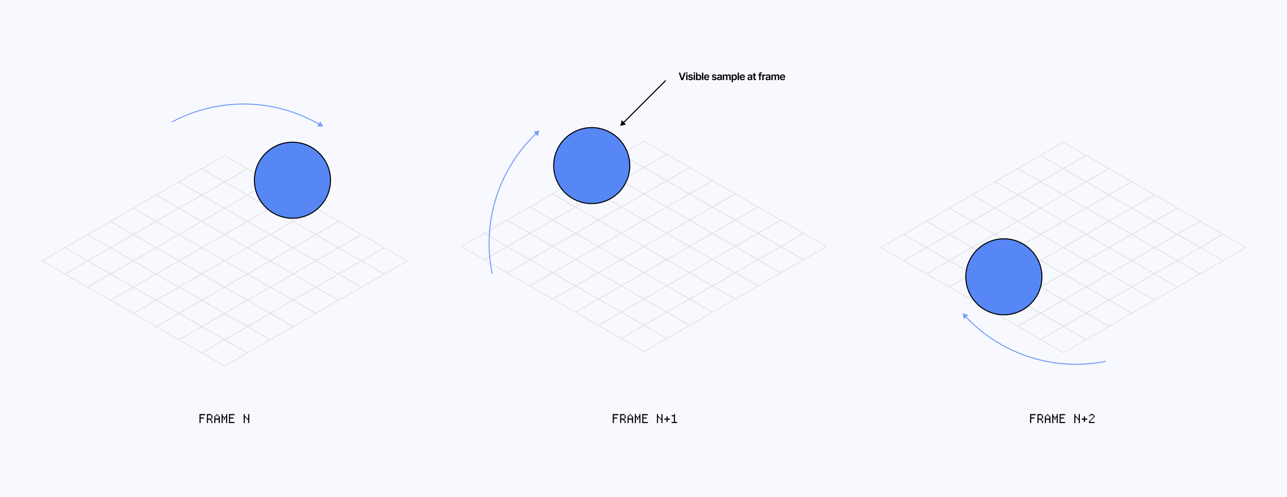
I was intrigued by this side-effect, especially after reading Pierre Cusa’s article titled Motion All the Way Down, where, among many other things, he introduces a hack to solve for it that I thought would fit well in our example here: rendering copies of our moving objects where we expect them to be.
Of course, this solution only works when the object follows a predictable trajectory that we can evaluate between frames. The code snippet below demonstrates this hack for our sphere’s circular trajectory.
Analytical solution to the wagon-wheel effect
1for (let index = 0; index < activeSmearSamples; index += 1) {2const smearSphere = smearSphereRefs.current[index];34// Sample each interval's center, then center the range on the current frame.5const phase = (index + 0.5) / activeSmearSamples;6const centeredPhase = phase - 0.5;7const smearAngle =8angle +9centeredPhase * delta * smearSpeed * SMEAR_EXPOSURE_WIDTH;1011// Evaluate the sphere's known circular trajectory at that time.12smearSphere.position.set(13Math.cos(smearAngle) * ORBIT_RADIUS,140,15Math.sin(smearAngle) * ORBIT_RADIUS,16);1718// Use a raised-cosine shutter weight so the trail fades at both ends.19const shutterWeight = 1 - Math.cos(phase * Math.PI * 2);20smearMaterial.opacity =21(shutterWeight / 2) *22objectSmearStrength *23smearVisibility *240.35;25}
As a result, we get more of the object’s movement between frames, which leaves a smooth trail along its path.
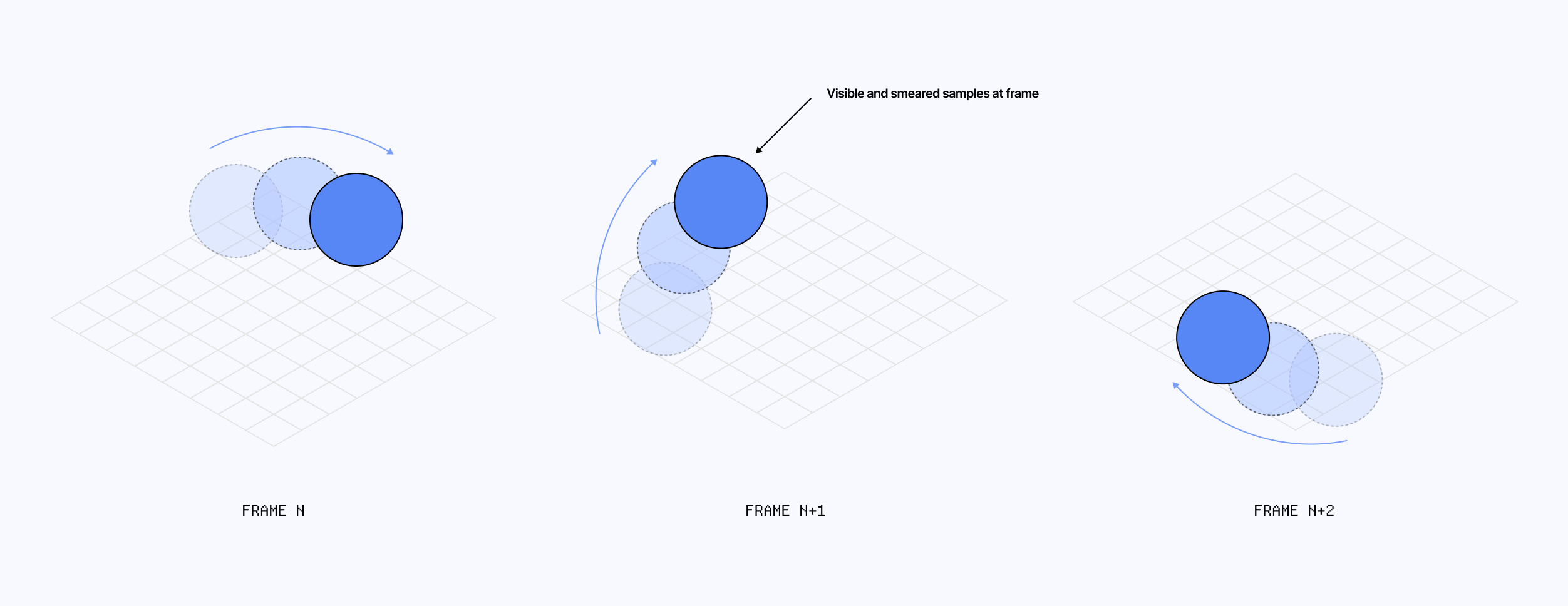
The next and final demo features this hack at work. I also included a weight to the opacity of the different copies so that samples close to the center, a.k.a. the real mesh, appear stronger. The effect is very satisfying and features some kind of recoil due to the trail expanding and contracting as the speed of the object gets changed. Take some time to play with it to get a good feel for it.
Again, this is a hack; there may be a more elegant solution to this issue, but this one was so smart and simple and produced such a lovely result that I had to share it. As a word of caution, I’d recommend the following 3 improvements before you think of shipping this to production:
- Only using this in a very limited use case, like here, one or two meshes.
- Reducing the number of vertices for the copies to avoid any potential performance impact this may have
- Maybe looking into using instances rather than discrete meshes (I was lazy here).
This article mainly stemmed from a personal challenge: to reproduce the effects I saw some of my friends, and many other creators, playing with on TouchDesigner or similar softwares, but on the web to give us a new outlook on what we can unlock in terms of interactivity and visual language when using motion.
Building these made me appreciate how, from a very simple set of techniques such as frame differencing, we managed to infer fairly complex and fine details such as what is moving in a given scene, how intensely, and in which direction. Once converted to luminance or flow map, we saw that motion can be interpreted the same way as color, light, or depth in many classic post-processing effects, allowing us to combine different aesthetics.
While the output is nice, I have yet to find a concrete application for blob tracking, optical flow, or motion blur beyond the simple detection or visual use case. Not that we necessarily need to focus our time only on algorithms and shading techniques to produce useful results, but I generally like to see where and how some of the pieces we looked into can fit in other contexts as part of a solution to a bigger problem. For now, the creative and visual aspect will have to be enough. It never hurts to dilly-dally a bit while learning without a set goal and see where it leads you.
Finally, I also want to shoutout @creativecodingnyc, who let me display some of the work featured here during one of their showcase in early June in Brooklyn.
We have also seen an example of decay used for an effect in Post-Processing Shaders as a Creative Medium to implement a mouse trail.
I shared more details about how I organize my WebGPU code in React Three Fiber, including compute shaders at Field Guide to TSL and WebGPU. It's also a great resource if you need a refresher on what compute shaders are and how they work.
A Signed Distance Function returns the shortest distance from a point to the edges of a shape. The resulting "sign" tells us whether a given point is inside or outside the given shape. We use these as a "drawing tool" when working with shaders.
I broke down the process of evaluating cubic bézier curves in Cubic Bézier: from math to motion. The formulas presented are the same as the ones we use in the shader code of our examples in this article.
A Sobel filter follows a similar process but uses weighted 3×3 kernels, producing a smoother and more robust estimate than our four-sample approximation.